A detailed explanation of the Poincaré sections of the swing-spring can be found in the book: Essentials of Hamiltonian Dynamics. With the aforementioned clarified, we can formulate the function to obtain the Poincaré sections of two-degree-of-freedom systems as follows:
Sections[eqns_?VectorQ, depvars_?VectorQ, cross_,
   retrievesec_?VectorQ, icv : {__?NumericQ}, tmax_Integer?Positive] /;
   Length[retrievesec] == 2 && Length[icv] == 4 := Module[{vars, time},
  time = Times @@ Variables@Level[depvars, {-1}];
  vars = Head /@ depvars;
  Reap[NDSolve[
     Join @@ {eqns,
       Thread[Through[vars[0]] == icv], {WhenEvent[cross,
         Sow[retrievesec, "LocationMethod" -> "EvenLocator"]]}},
     vars, {time, 0, tmax}, MaxSteps -> \[Infinity],
     MaxStepSize -> 0.1]][[-1, 1]]]

Sections[eqns_?VectorQ, depvars_?VectorQ, cross_,
  retrievesec_?VectorQ, icv_?MatrixQ, tmax_Integer?Positive] :=
 Map[Sections[eqns, depvars, cross, retrievesec, #, tmax] &, icv]
Next, an example with a set of 67 initial values is provided:
hameqns = {x'[t] == px[t],
   px'[t] == x[t] (-4 + 3/Sqrt[x[t]^2 + (-1 + y[t])^2]),
   y'[t] == py[t],
   py'[t] ==
    3 - 3/Sqrt[
     x[t]^2 + (-1 + y[t])^2] + (-4 + 3/Sqrt[
        x[t]^2 + (-1 + y[t])^2]) y[t]};
states = {x[t], px[t], y[t], py[t]};
cross = x[t];
retrievesec = {y[t], py[t]};
icvals = {{0, 1.2058438021483298`, 0.23435349229150537`,
    0.07908531737029979}, {0, 1.053859439927374, 0.3380893192713096,
    0.3349070462898792}, {0, 1.0312212764574027`,
    0.34979954074206077`, 0.35657229865503887`}, {0,
    1.0242197558040889`, 0.3570487254620496,
    0.34790619770897496`}, {0, 1.018972754357531, 0.362542732311133,
    0.3405078484712786}, {0, 1.0707993739458272`, 0.3313977641451661,
    0.30674221821517167`}, {0, 1.1087584210261923`,
    0.30965020998519954`, 0.2590786630118205}, {0,
    1.1244974141573785`, 0.2976757449936718, 0.2471076059598717}, {0,
    1.137507616780038, 0.28918896199066574`, 0.2270581397317511}, {0,
    1.1528934238004025`, 0.2770002349339941,
    0.20957154564452146`}, {0, 1.1578556873638288`,
    0.2724159544549544, 0.20622414570757833`}, {0, 1.157377501246667,
    0.28088353647356945`, 0.15778173329135867`}, {0,
    1.1547745755595673`, 0.2875626765126868,
    0.12540537448076486`}, {0, 1.150289624179014,
    0.29484901110081474`, 0.09534161272807058}, {0, 1.143897452400374,
     0.30274254023795344`, 0.06990304509117545}, {0,
    1.138752682805667, 0.3088144857280601, 0.04215188039638076}, {0,
    1.1367634704827951`, 0.31124326392410273`,
    0.016713312759485625`}, {0, 1.1354248192294862`,
    0.312574144733999, -0.00030992406241277075`}, {0,
    1.1561714734989113`, 0.2620605054542388,
    0.26184860089683876`}, {0, 1.151850600146605,
    0.25142907909040346`, 0.31681835125654}, {0, 1.1482860214864978`,
    0.2398335862945928, 0.3624342925262546}, {0, 1.14232840004029,
    0.22504968576356899`, 0.41532683781844243`}, {0,
    1.193089824441555, 0.16876003351902275`, 0.3776464949667249}, {0,
    1.1787250029993586`, 0.15642196545850912`,
    0.4390171320034674}, {0, 1.155900241021198, 0.14257201231398256`,
    0.5124329400283544}, {0, 1.2923447648782078`,
    0.049262492930158656`, 0.01174035149020717}, {0,
    1.2947319550530585`, 0.030284768457285095`,
    0.0007041039979025152}, {0, 1.2956372075678675`,
    0.016176805918764255`, -0.016657435781195253`}, {0,
    1.0979892706910315`, 0.06470015820472003, 0.676516902642139}, {0,
    1.0620094611198883`, 0.0803287233402036, 0.7254826595570544}, {0,
    0.9630052282829985,
    0.18191439672084686`, -0.7875592291138307}, {0,
    0.8795034213364558, 0.15977392944557847`, 0.8968628087592583}, {0,
     0.8234519661738053, 0.15977177331636275`,
    0.9485877825535564}, {0, 0.16499650468939198`,
    0.058220869490935245`, 1.2803192862966493`}, {0,
    0.5704504945083201, 0.08558915428104083, 1.1512098939780868`}, {0,
     0.030938085724460513`, 0.6259776498931662,
    0.3341418294506401}, {0, 0.9696312807190509, -0.06500353876792028,
     0.8502431059654192}, {0,
    0.7481542774429455, -0.11957763987424194`, 1.031052825665227}, {0,
     0.8791408122636859, -0.21402189428041013`,
    0.8508172231959377}, {0,
    0.7769950861417774, -0.24826777647783269`,
    0.9108957573523677}, {0,
    0.7872147314780307, -0.20912570761613247`,
    0.9409350244305815}, {0,
    0.8287838648279349, -0.17250252918354192`,
    0.9349271710149386}, {0, 0.9018523759517163, -0.1634763438473578,
    0.8716445559971367}, {0, 0.8663003040147248, -0.2328173043478992,
    0.8442204655471852}, {0, 0.783789988332275, -0.2508097613002086,
    0.9022478089395519}, {0, 0.6723615259663238, -0.3020922374834779,
    0.9289193175992956}, {0,
    0.9032324190828922, -0.27955489690957597`,
    0.7426758617143631}, {0, 0.9409679938672925, -0.2936407347682647,
    0.6705816207266473}, {0, 1.1538948621555278`, -0.2739205617661005,
     0.21999261455342337`}, {0,
    1.1430559564856309`, -0.2964579023400024,
    0.14789837356570754`}, {0, 1.12494435212768, -0.3218124104856421,
    0.015725598421561876`}, {0,
    1.081485423648365, -0.34434975105954396`,
    0.18995334747520845`}, {0,
    1.0601187670840475`, -0.34434975105954396`,
    0.2860790021254962}, {0, 1.0246373023906838`, -0.3640699240617082,
     0.3161182692037111}, {0,
    0.8055273194560775, -0.43793253633320695`,
    0.5137957883176585}, {0,
    1.1794745332678316`, -0.23870596711937875`,
    0.24681505306410922`}, {0, 0.912496162101068, -0.4288647782116761,
     0.3341418294506401}, {0, 0.9110540599894742, -0.4401334484986271,
     0.27406329529421025`}, {0,
    0.9175565040484254, -0.44576778364210257`,
    0.2079769077221374}, {0,
    0.9059710770307129, -0.45703645392905357`,
    0.15390622698135054`}, {0,
    0.8916551566262928, -0.4683051242160045, 0.0878198394092777}, {0,
    0.8808161244041481, -0.47543632485894777`, \
-0.0020393646374972096`}, {0,
    1.058493203560303, -0.29645790234000235`, -0.4561172947579481}, \
{0, 0.40186625466347564`, 0.18527775242715105`,
    1.175241307640658}, {0, 0.472823848474096, 0.13741430764934137`,
    1.1751199260191079`}, {0, 0.9006450150678906,
    0.17685608016817767`, 0.8623956542466731}, {0,
    1.1227397919762903`, -0.16667716084363393`, \
-0.5552749370586232}};
tmax = 5000;
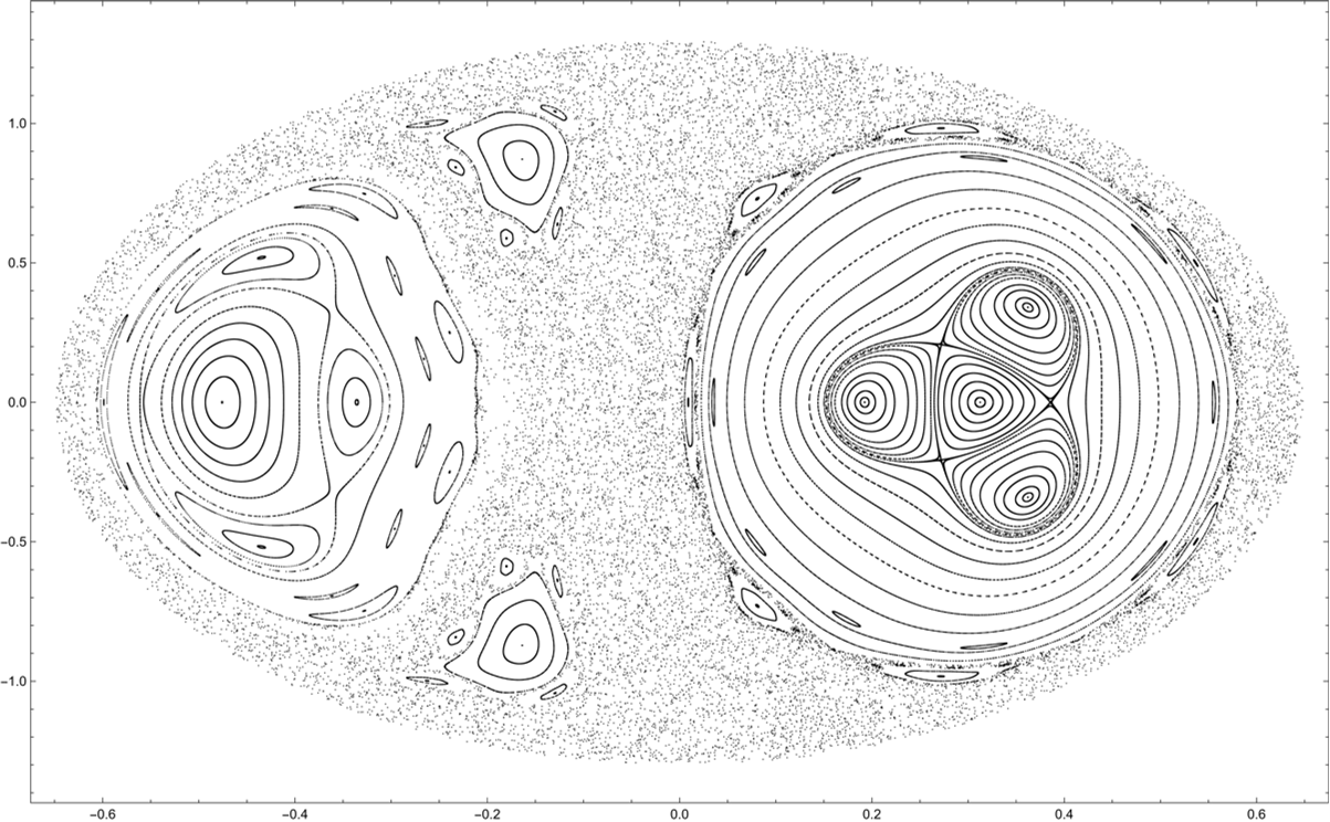
The Poincaré section for the given initial conditions appears as follows:
ListPlot[Sections[eqns, states, cross, retrievesec, icvals, tmax],
 PlotStyle -> {{AbsolutePointSize[0.5], Black, Opacity[0.7]}},
 ImageSize -> Full, Frame -> True, FrameStyle -> Directive[Black],
 Axes -> False]