
Real-Time Detection of Daytime and Night-Time Fire Hotspots from Geostationary Satellites


1
STEM College, RMIT University, Melbourne, VIC 3000, Australia
2
Bushfire and Natural Hazards Cooperative Research Center, East Melbourne, VIC 3002, Australia
*
Author to whom correspondence should be addressed.
Remote Sens. 2021, 13(9), 1627; https://doi.org/10.3390/rs13091627
Submission received: 3 March 2021
/
Revised: 8 April 2021
/
Accepted: 9 April 2021
/
Published: 21 April 2021
Abstract
:This paper introduces an enhanced version of the Biogeographical Region and Individual Geostationary HHMMSS Threshold (BRIGHT) algorithm. The algorithm runs in real-time and operates over 24 h to include both daytime and night-time detections. The algorithm was executed and tested on 12 months of Himawari-8 data from 1 April 2019 to 31 March 2020, for every valid 10-min observation. The resulting hotspots were compared to those from the Visible Infrared Imaging Radiometer Suite (VIIRS) and the Moderate Resolution Imaging Spectroradiometer (MODIS). The modified BRIGHT hotspots matched with fire detections in VIIRS 96% and MODIS 95% of the time. The number of VIIRS and MODIS hotspots with matches in the coincident modified BRIGHT dataset was lower (at 33% and 46%, respectively). This paper demonstrates a clear link between the number of VIIRS and MODIS hotspots with matches and the minimum fire radiative power considered.

1. Introduction
Data from multi-channel satellites, carrying instruments that observe mid-infrared (3–8 µm; hereafter MIR) and thermal-infrared (8–15 µm; hereafter TIR) bands can be used to detect fires. In the absence of cloud, an increase in MIR (compared to some representative value), along with an increase in MIR minus TIR can indicate fire [1]. While many satellites can be used to detect fire, their orbits, along with the specific characteristics of their instruments, impact the sensitivity and frequency of their fire detections. For large and fire-prone continents such as Australia, the sensitivity, frequency, and timeliness of satellite fire surveillance is critical for the detection, monitoring. and tracking of fires. As the instruments carried onboard satellites have evolved, satellite fire surveillance has become more sensitive, frequent, and timely.
Satellite instruments differ in terms of the number of bands they observe, their central wavelengths (and response functions), and orbital characteristics. Instruments carried onboard Low Earth Observation (LEO) and Very Low Earth Observation (VLEO) satellites systematically observe the globe, with specific locations typically observed no more than two times per day. Cross-over times are not optimized for fire detection (i.e., late afternoon fires in Australia) [2,3]. Instruments onboard LEO and VLEO satellites used to detect fire include the Advanced Very High Resolution Radiometer [4,5,6,7,8], Visible Infrared Imaging Radiometer Suite (VIIRS) [9,10], Moderate Resolution Imaging Spectrometer (MODIS) [11,12,13,14], and Bi-spectral InfraRed Detection Hot Spot Recognition System [15,16]. Instruments onboard Geostationary Earth Observation (GEO) satellites scan broad spatial regions (full-disk), but with a lower spatial resolution (compared to contemporary LEO systems). Repeated scans from GEO instruments ensure updates within minutes (instead of 12 or more hours). Instruments onboard GEO satellites used to detect fire include the Visible Infrared Spin Scan Radiometer Atmospheric Sounder [17], different versions of the Geostationary Operational Environment Satellite Imager [18,19,20,21,22,23], the Advanced Baseline Imager [24,25], the Spinning Enhanced Visible and Infrared Imager [26,27,28,29,30], and the Advanced Himawari-Imager (AHI) [31,32,33,34]. While the higher spatial resolution of data from LEO and VLEO satellites can be an advantage for detecting smaller and/or lower intensity fires, the lower spatial resolution of data from GEO satellites can be an advantage when tracking and characterizing the properties of stronger fires. Hence, fire information from LEO, VLEO, and GEO satellites can complement each other.
The pixel size of satellite observations impact the fire brightness temperatures recorded and are linked to the fire size and intensity, which are can be retrieved through fire detection algorithms. Current variations in pixel sizes (such as (at ~4 µm) AHI/Himawari-8 2 km, MODIS/Terra 1 km and VIIRS/Suomi-NPP 375 m resolution) mean that fire brightness temperature will differ between satellite and instrument combinations. For example, for MIR readings below 350 K in [13,14], fires were detected using statistics, with potential fire pixels compared to samples of data. Data samples typically need to be fire-free for statistically-based fire detection algorithms as samples derived from fire-affected data may cause missed detections. Data samples also typically need to be cloud-free as clouds can block outgoing radiation, reflect sunlight, and/or artificially lower statistics [1]. Cloud detection algorithms are also sensitive to pixel size [35], and gross checks for fire and/or cloud in data samples are likely to degrade with increases in satellite pixel size. Hence, the quality of ancillary information such as cloud masks (and coarse fire thresholds) can impact the design of fire algorithms, with workarounds required when they are not available [32,34].
Routine scans of the full disk from GEO satellite instruments create an abundance of data for use in statistics. Such data allows for a new generation of fire detection algorithms [33,34]. Traditional LEO contextual algorithms compare potential fire pixels to cloud-free and fire-free pixels from spatiotemporally similar data (data within the same scan and within a given area typically defined using expanding boxes) [4,13,14]. Some GEO algorithms define data samples similarly [17,19,24,27,28]. Larger temporal windows of data are used for cloud-detection in [21,32], but the same scan (spatially co-located using a similar methodology outlined in [13,14]) is then used for fire detection. The concept of multi-day temporal data for fire detection for LEO data was used in [36,37], while [25] used multi-day regression for fire detection in GEO data. Single value decomposition temperature fitting (using up to thirty days of prior data for training data) was used in [29,33] to detect fires in GEO data. While sophisticated cloud-detection algorithms developed for LEO data [38,39] could be adapted to GEO data, they were not considered here due to the additional lag-time they could introduce to the computation of active-fire hotspot detections.
Recently, an algorithm was proposed that combined concepts of biogeographical regionality, seasonality, and time-of-day to detect fires in cloud- and fire-affected GEO data [34]: Biogeographical Region and Individual Geostationary HHMMSS Threshold (BRIGHT). BRIGHT derived biogeographical, seasonal, and time-of-day statistics from GEO data, allowing adaptive thresholds to be determined and fires to be detected—despite cloud-mask (and fire-masking) information being unavailable. The simplicity of the algorithm permitted the research to be done easily at scale, with a 12-month, Australia-wide study conducted. BRIGHT hotspots were found to match the MODIS hotspots 88% of the time. While MODIS hotspots were found to match with coincident BRIGHT hotspots only 39% of the time, the undetected MODIS hotspots were shown to have low radiative power [34]. However, the algorithm was restricted to post-event analysis during the daytime.
This paper details the work undertaken to adapt the BRIGHT algorithm to make it capable of working continuously in real-time over daytime and night-time conditions. The algorithm utilizes a rolling window (rather than a fixed sub-seasonal definition) with instantaneous final MIR statistics rather than a sub-seasonal estimation. The algorithm was tested on 12-months of AHI/Himawari-8 data, with the period including the catastrophic Black Summer fires that occurred in 2019/2020 in southeast Australia. The resulting active fire detections were compared to those from the MODIS and VIIRS fire detection systems. Fire burning patterns were explored, along with the number of matches.
2. Materials and Methods
2.1. Study Area and Data
The Australian continent was chosen as a case study area due to its large size (over 7.6 million km2) and biogeographically diverse areas. Regions across Australia were defined using the Interim Biogeographic Regionalization for Australia (IBRA) sub-regions [40]. In total, there were 419 IBRA sub-regions. Higher level aggregation into IBRA bioregions, referred to in this paper as biodomains, were also used. In total, there were 89 IBRA biodomains.
AHI/Himawari-8 [31] 0.64 µm (channel #3) (reflectance; hereafter
), 3.9- (), and 10.4 µm () brightness temperature (channels #7 and #13) values were used at 2 km resolution every 10-min over Australia to execute the algorithm. An ancillary AHI/IBRA reference grid was produced to assign all AHI pixels to one of the 419 IBRA sub-regions. From this, BRIGHT hotspots were produced from the AHI dataset for 12-months starting 1 April 2019 and ending on 31 March 2020 (inclusive).
Archival quality MODIS (Collection 6) and VIIRS hotspots were downloaded from the Fire Information for Resource Management System (FIRMS) website (https://firms.modaps.eosdis.nasa.gov/, accessed on 2 October 2018) for comparative purposes. MODIS hotspots from 1 April 2019 to 30 September 2019 were downloaded on 15 January 2020, while MODIS hotspots from 1 October 2019 to 31 March 2020 were downloaded on 27 July 2020. VIIRS hotspots from 1 April 2019 to 31 March 2020 were downloaded on 24 September 2020. FIRMS hotspots were restricted to those with an along scan pixel size multiplied by the along track pixel size value of less than 1.7 km [32,34] and a presumed vegetation fire inferred hot spot type. FIRMS hotspots were assigned the nearest AHI scan time (after the hotspot) and AHI pixel location prior to further processing.
2.2. Algorithm Overview
Here, a new algorithm is introduced that extracts geostationary satellite data for a relevant biogeographical region, for the current day and the 28 days preceding. Dynamic thresholds are calculated using full or partial samples depending on the variable being investigated. The thresholds are then used to determine active fire hotspots (see Figure 1 for an overview of the modified BRIGHT algorithm).
2.3. Prepare Geostationary Satellite Data
For the given biogeographic regions (R), consider all pixels with number identifier R, in other words,
where I2 is the set of all AHI full-disk vertices, and B is a reference grid with each geostationary satellite data pixel assigned to a specific biogeographical region.
“Day” or “night” categories are assigned using reflectance data. Active fire algorithms use different equations for daytime and night-time [13,14]. The real-time BRIGHT algorithm defines the day or night period using reflectance data. The geographic region of interest is defined as a box that encapsulates all pixels, plus the surrounding 50 pixels. If any row of reflectance data (within the box) has more than nine invalid pixels, the region is assigned to the “night” category. Otherwise, the region is assigned to the “day” category. While day/night assignments may be more robust using solar zenith angle, the method described was chosen due to the speed of processing to enable faster delivery of active fire information to resource managers. Once the day/night assignment is complete, data are then collected as follows.
For the date and time combination ts, consider all times in the set T, with T defined as
For each time t in T, take the , , and matrices and construct a set of spatiotemporally co-located variables D(t) specific to time t and region R, with:
2.4. Determine Thresholds
Thresholds for , , and are processed separately with some results feeding into subsequent calculations (Figure 2). Bearing in mind the order of processing, , , and thresholds were calculated using the five steps shown in Figure 3: filtering, clipping, comparing, size checking, and the final threshold calculation.
During the day, if V denotes , , or the filtered data are:
where the condition C(V) is
During the night, if V denotes or the filtered data are
where the condition C(V) is
The
and terms are the data-defined reflectance and TIR threshold calculated using reflectance and TIR data (defined later in this section).
Each set-member is clipped with:
where means the Xth percentile of the set, and
and
A set of median values (M) is created, with
Clipped set members are then compared, with clipped set members discarded if their corresponding value falls above or below .
If the variable is , or , the remaining set members are compared again using the set of inter-quartile range (IQR) values I, with
Set members are discarded if their corresponding I(t) value fall above or below .
Multi-day thresholds are then used for during the day and during the night. Multi-day thresholds are calculated by collapsing all the remaining members into one sample. during the day is calculated using a histogram of values binned in 0.03 BRF bins from 0 BRF to 0.33 BRF (as in [24]). The is defined using the edge of the maximum bin + 0.06 (with a maximum 0.33 value). The multi-day thresholds during the night are calculated = S25th − 1.0 (S75th − S25th) and as the median of the collapsed sample.
Single-day thresholds are used for all remaining thresholds, based on the remaining data from the current day alone (). If after prior screening had less than 30% of the original raw data sample size (for that one day), an invalid threshold is recorded. Otherwise, single-day thresholds are calculated as follows.
Current-day BRIGHT statistics are derived as
and
or
2.5. Hotspots
During the day, pixels in D(t0) are considered as fire if either condition (17) or conditions (18)–(20) are met, along with (21) and (22) with R = 5-, 7-, 15 K, respectively, and (17)–(22) are defined as follows:
During the night, pixels in D(t0) are considered fire if either condition (23) or conditions (24), (25) and (26) are met, with conditions (23)–(26) defined as follows.
In the absence of a valid sample size, only conditions (17) or (23) apply.
2.6. Confidence
To assign confidence levels, conditions (27) and (28) were defined as:
Hotspots that satisfied either (17) or (23) were assigned an absolute threshold indicator (ABS). Hotspots that did not satisfy (17) or (23) were assigned a lower confidence (LO) if they satisfied (27) and (28), and a higher confidence (HI) otherwise.
3. Results
3.1. Continental Comparison
BRIGHT (AHI/IBRA) hotspots were compared to VIIRS and MODIS hotspots predicated by the assumption that those sources with a higher spatial resolution provided the more accurate dataset. VIIRS and MODIS swaths were reconstructed using the methodology defined in study [34]. The process is summarized here for clarity. Hotspots from VIIRS or MODIS with the same observation time were used to define a reconstructed swath box (for that one sensor). BRIGHT hotspots that fell within that box, and within +/− 10 min were compared to the reconstructed swath hotspots. Hotspots were declared “matched” if one or more hotspots from the opposing dataset were found within +/− 1 pixel, otherwise the hotspot was declared “unmatched”.
Duplicates were defined as hotspots with the same sensor, time, and location, but included in different swath reconstructions. Duplicate hotspots were counted only once. A hotspot was counted as “matched” if the hotspot was designated as “matched” in any reconstructed swath (this process compensates for sub-optimal VIIRS swath reconstructions).
The pixel sizes for AHI, MODIS, and VIIRS at ~4 µm differ. The channel closest to 4 µm has 2 km spatial resolution for AHI, 1 km for MODIS and 375 m for VIIRS. An AHI pixel would cover the same area as roughly four MODIS pixels, or 25 VIIRS pixels. The variation in spatial resolution for a given pixel affects the rise in radiance above that of the thermal emission coming from Earth, and hence the sensor/algorithm sensitivity. The impact of a sensor’s spatial resolution on the number of matches are discussed in the following sections.
BRIGHT-to-VIIRS and BRIGHT-to-MODIS comparisons were assessed in terms of BRIGHT-to-LEO(BRIGHT) and BRIGHT-to-LEO(LEO) unmatched hotspots. The BRIGHT-to-VIIRS (BRIGHT) and BRIGHT-to-MODIS (BRIGHT) comparisons had 4% and 5% unmatched hotspots for the day and night hotspots combined (Table 1). In contrast, BRIGHT-to-VIIRS (VIIRS) and BRIGHT-to-MODIS (MODIS) comparisons had 67% and 54% (Table 1) unmatched hotspots for day and night hotspots combined, respectively.
3.2. Unmatched LEO Hotspots
Fire radiative power (FRP) values indicate the amount of energy being released by wildfires by comparing the brightness temperature of the fire-affected pixel to that of a cloud-free and fire-free representative pixel [15]. The amount of energy released affects whether a fire is detectable or not for a given pixel size. The number of VIIRS/MODIS hotspots decreased non-linearly with rising minimum FRP value (as reported in FIRMS) (Figure 4, solid black lines). The same was true for the sample containing only hotspots with a valid BRIGHT threshold (Figure 4, solid blue lines). As the minimum FRP increased, so did the probability of detection (POD). Higher PODs at higher minimum FRPs (Figure 4; all hotspots (dashed black lines); hotspots with valid BRIGHT thresholds (dashed blue lines)) suggested that BRIGHT had greater utility in detecting stronger fires, although the significant difference in sample sizes should also be considered. When considering only hotspots with a valid BRIGHT threshold PODs were greater than 80% at 55 MW (MODIS-day), 44 MW (VIIRS-day), 16 MW (MODIS-night), and 15 MW (VIIRS-night) (Figure 4; dashed blue lines, red circles and accompanying text).
During the day, 99% of unmatched MODIS hotspots had AHI values below the level of detection. The high-frequency full-disk AHI observations allowed for AHI values to be obtained at ALL MODIS hotspot times and locations. AHI and BRIGHT values were obtained at all unmatched MODIS hotspot locations (Figure 5). Unmatched MODIS hotspots with BRIGHT < 5 were undetectable with the current algorithm settings (due to conditions (22) and (25)). While conditions (22) and (25) can be relaxed, potential false alarms need to be considered (see next section). A total of 17,129 (3110) unmatched MODIS hotspots had no valid BRIGHT threshold during the day (night). During the day, only 263 out of 28,628 (<1%) of the remaining unmatched MODIS hotspots had AHI values with BRIGHT < 5. During the night, 1136 out of 11,532 (10%) unmatched MODIS hotspots had AHI values that satisfied condition (25). The remaining sample failed the other algorithmic thresholds.
3.3. Disagreements during Burning Periods
Hotspot counts were collated for individual biodomains (using ancillary IBRA information) and calendar months. Counts were calculated for all BRIGHT-to-VIIRS, BRIGHT-to-MODIS daytime (night-time) combinations. The results were sorted in descending order, according to the number of raw hotspots. Biodomain identifiers were then collected until at least 50% of the raw hotspot activity (for each BRIGHT-to-VIIRS, BRIGHT-to-MODIS, day/night combination, separately) were accounted for. The biodomain identifiers were reduced to one set (Figure 6; white and grey regions). The counting and sorting processes were repeated for unmatched hotspots. The unmatched hotspot regional identifiers included most of the raw fire activity regions, plus some additional ones (Figure 6; white and pink regions; for a description of the biodomains see Figure 6).
The biodomains were grouped into spatial regions (southeast, southwest, central-north, and northeast Australia) against which raw and unmatched counts per month were plotted (see Figure 7 and Figure 8). The monthly patterns remained relatively stable within each of the four distinct spatial biodomains, but varied between them.
The fire activity in southeastern Australia (BBS, SEQ, NET, NNC, SYB, SEC, and SEH; Figure 6) began in September 2019 and continued through to February 2020. The peak fire activity occurred in the Sydney Basin during December 2019 for all comparisons. BRIGHT-to-VIIRS (VIIRS) (Figure 7a), and BRIGHT-to-VIIRS (BRIGHT) (Figure 7c) showed similar patterns of daytime fire activity in southeastern Australia, however, BRIGHT-to-VIIRS (BRIGHT) had lower raw counts (Figure 7c, see color bar). The same can be said for the BRIGHT-to-MODIS comparison (Figure 7e,g). Night-time BRIGHT-to-VIIRS (VIIRS) raw counts were higher than daytime BRIGHT-to-VIIRS (VIIRS) raw counts (Figure 7a versus Figure 8a). While night-time BRIGHT-to-MODIS (MODIS) raw counts were lower than daytime BRIGHT-to-MODIS (MODIS) raw counts (Figure 7e versus Figure 8e). Hence, VIIRS and MODIS may differ in their respective daytime/night-time sensitivity.
The per-month unmatched counts for southeastern Australia were also informative. The BRIGHT-to-VIIRS (VIIRS) and BRIGHT-to-MODIS (MODIS) per-month unmatched hotspot counts had patterns that reflected the raw hotspot counts (Figure 7a,b,e,f): note the high level of maximum unmatched hotspot counts. This is consistent with the BRIGHT-to-VIIRS (VIIRS) and BRIGHT-to-MODIS (MODIS) unmatched hotspots discussed in Section 3.2; but shows that the omitted hotspots were spread across the burning periods and were not concentrated in one biodomain/month combination. In Figure 7d,h and Figure 8d,h, apart from AUA, SVP, SEQ, and NSS (which will be discussed in the next section), the BRIGHT-to-VIIRS (BRIGHT) and BRIGHT-to-MODIS (BRIGHT) per-month unmatched counts were significantly lower (max 200) and occurred during times of high raw counts (across all sensor combinations). These results indicate that some of the BRIGHT-to-VIIRS (BRIGHT) and BRIGHT-to-MODIS (BRIGHT) unmatched hotspots may have occurred during times of high fire activity and may signify disagreement rather than outright error.
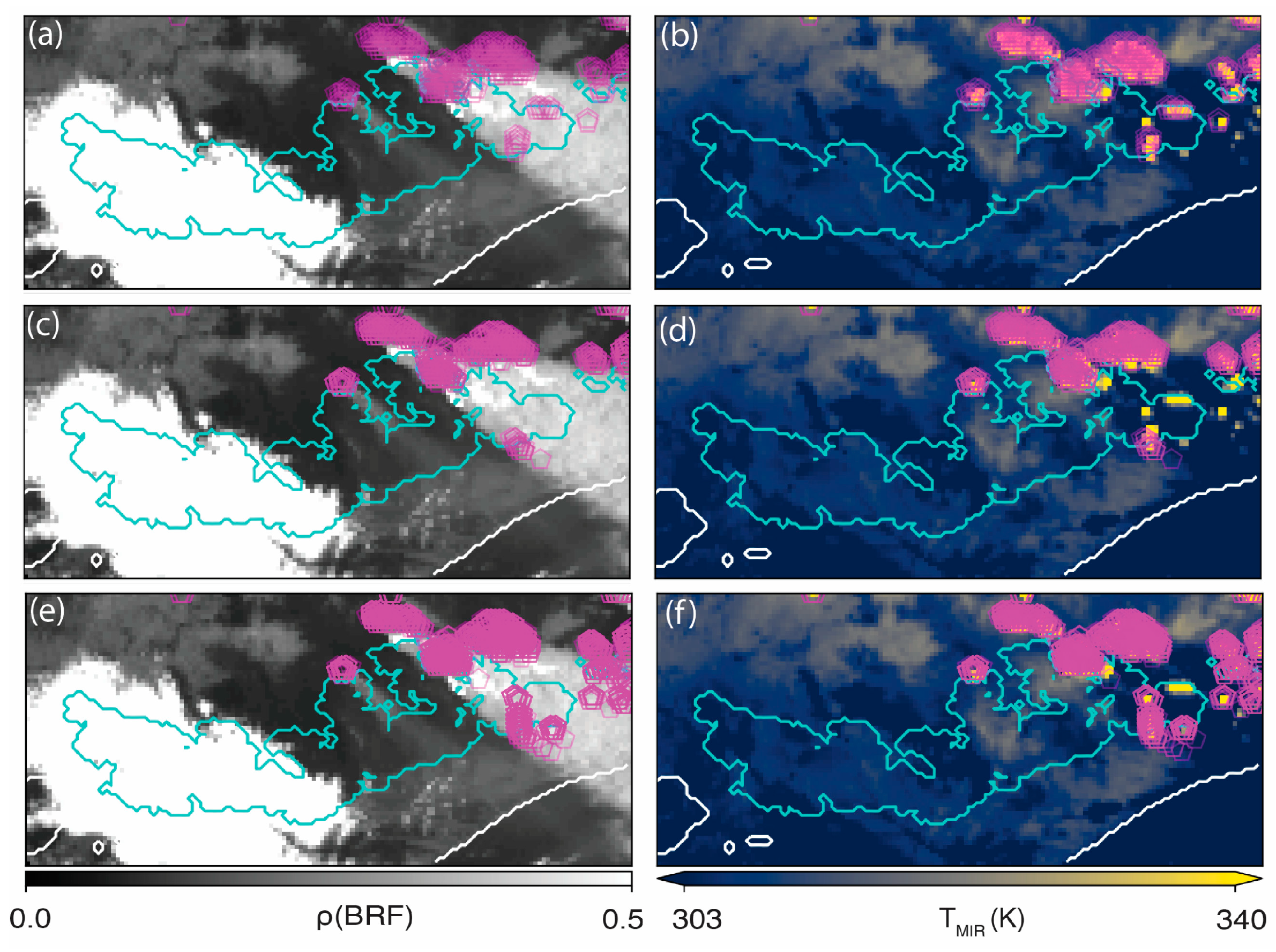
Figure 9 shows an example of disagreements during high fire activity. In the SEH01 region (within biodomain SEH; Figure 6) BRIGHT, MODIS, and VIIRS fire detections are shown when both MODIS and VIIRS were crossing Australia at the same time (04 UTC 4 January 2020). While all three satellites detected fires, there were differences most likely due to the heavy smoke occurring at that time. In this example, the BRIGHT algorithm was capable of detecting fires in areas covered with heavy smoke/cloud due to SEH01 thresholds calculated using the remaining cloud-free and smoke-free data in the SEH01 region on that day at that timepoint (Figure 9, aqua outline, SEH01 includes both clear and cloudy data).
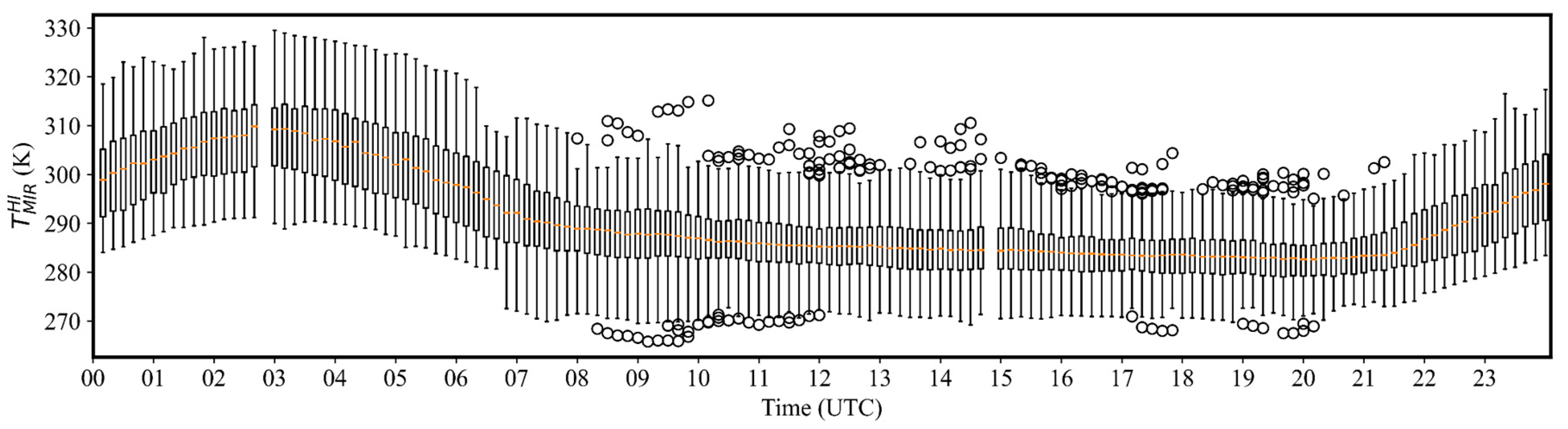
Furthermore, Figure 10 demonstrates how dynamic the BRIGHT SEH01 BRIGHT thresholds were. BRIGHT thresholds for region SEH01 varied significantly within each AHI timepoint, with noticeable differences between AHI timepoints in line with the diurnal cycle. Other regions (not shown) also demonstrated similar levels of variability. The variance of the BRIGHT thresholds highlight the dynamic nature of the BRIGHT algorithm.
The fire activity in southwestern Australia (GVD and COO; Figure 6) occurred during similar months as southeastern Australia, but with less intensity (i.e., VIIRS, MODIS, and BRIGHT had similar patterns of fire activity, but with lower raw counts comparatively). The BRIGHT-to-VIIRS (BRIGHT) and BRIGHT-to-MODIS (BRIGHT) unmatched counts again peaked in times of high raw counts for all sensor combinations.
The burning patterns of north-central Australia differed in intensity and monthly pattern. North-central Australia had consistent fire activity from April 2019 to December 2019. For NOK, VIB, PCK, DAC, CEA, and ARC (Figure 6), the burning patterns of VIIRS, MODIS, and BRIGHT were similar, with BRIGHT peak raw counts lower than those of VIIRS or MODIS.
Finally, in northeastern Australia, Cape York Peninsula (CYP) had a prolonged fire season, while Gulf Plains (GUP) had fires that occurred mainly in December 2019 (Figure 6, Figure 7 and Figure 8). Einasleigh (EIU) also had fires that occurred mainly in December 2019 though it only made the top 50% unmatched counts at night-time (Figure 6 and Figure 8). Cape York Peninsula (CYP) dominated the raw and unmatched counts for BRIGHT-to-VIIRS (VIIRS) during the daytime (Figure 7a,b). Cape York Peninsula (CYP) had similar fire burning patterns in BRIGHT-to-MODIS (MODIS) and BRIGHT-to-VIIRS (VIIRS) (during the daytime), but with lower raw counts (Figure 7e,f). The BRIGHT-to-VIIRS (BRIGHT) and BRIGHT-to-MODIS (BRIGHT) patterns were again similar to those of BRIGHT-to-VIIRS (VIIRS) and BRIGHT-to-MODIS (MODIS), but with lower raw counts (Figure 7 and Figure 8). BRIGHT-to-VIIRS (BRIGHT) and BRIGHT-to-MODIS (BRIGHT) peak unmatched counts Figure 7d,h and Figure 8d,h occurred at the same time as the peak BRIGHT-to-MODIS (MODIS) and BRIGHT-to-VIIRS (VIIRS) total counts Figure 7a,d and Figure 8a,d.
The biodomains with high levels of raw or unmatched hotspots over the entire time period varied between day (Figure 6a) and night (Figure 6b). Across daytime (night-time), at least 50% of the fire activity occurred in 16 (10) biodomains. Over 50% of the unmatched hotspots fell within 13 (9) of those biodomains, plus an additional three (three) biodomain (s). The night-time fire activity of north-central Australia was concentrated in less biodomains than in the daytime) (Figure 6, Figure 7 and Figure 8).
Note that AUA, SVP, and SEQ were included for high unmatched activity only in the daytime (AUA, EIU, and GUP for night-time); these will be discussed in the following section).
3.4. BRIGHT Confidence Measures
PODs varied with the confidence measures as defined in Section 2.6. When fires cause high satellite brightness temperatures, they can be detected using simpler measures (as in Equations (17) and (23)). Otherwise, detecting the fires requires thresholds and Equations (18)–(22) or (24)–(26). Analysis of PODs according to whether an outright threshold ((17) or (23)) was used, or if fire stood out strongly or weakly against the thresholds (Section 2.6; ABS, HI, and LO definitions) gave a different indication of the performance of the BRIGHT algorithm according to fire size and characteristics. There were 69,759 BRIGHT-to-VIIRS (BRIGHT) daytime hotspots: 27% ABS, 72% HI, and 1% LO. Of the 18,814 ABS hotspots, 96% had a match within the VIIRS dataset. Out of the 50,090 HI hotspots, 95% had a match with the VIIRS dataset. Of the 855 LO hotspots, only 16% had a match within the VIIRS dataset (see Table 2). Hence, BRIGHT hotspots with higher confidence (ABS or HI) had higher PODs.
To investigate further, the BRIGHT-to-VIIRS (BRIGHT) and BRIGHT-to-MODIS (BRIGHT) biodomains included in the top 50% unmatched counts (Section 3.3) were analyzed by region (for a description of regions and biodomains, see Section 2.1). Of those regions, the ones with the highest unmatched counts and less than 70% matched counts (and a minimum of 30 counts) were chosen for further analysis. The problematic regional subset included the Victorian Volcanic Plain (SVP01), Victorian Alps (AUA02), Barrington (NNC13), and Brisbane-Barambah Volcanics (SEQ05). Please note that the first three letters in the region correspond to the biodomain. For a spatial understanding of the relevant biodomains, see Figure 6.
The problematic region sample had a lower POD than the Australian sample. For BRIGHT-to-VIIRS (BRIGHT), the problematic regions together had 849 HI and 525 LO hotspots. The HI hotspots had a POD of 69%, and LO hotspots had a POD of 2%. The problematic regions alone accounted for 525 out of the 855 BRIGHT-to-VIIRS (BRIGHT) LO unmatched hotspots (Table 2).
The problematic regions stand out in terms of their sizes and/or the non-uniformity of their landscapes. The Victorian Volcanic Plain (SVP01) is 23.6 thousand km2 and is dominated by volcanic deposits, with unmatched BRIGHT hotspots occurring near urban areas [41] (Figure 11). The Victorian Alps (AUA02) is 5.2 thousand km2, and is both mountainous and discontinuous. Barrington (NNC13) is 1.1 thousand km2 with a sharp boundary between forested and cleared areas including the Barrington Tops National Park within it. Brisbane-Barambah Volcanics (SEQ05) is eight thousand km2 with 60% artificial and highly modified and 38.3% riverine areas. The LO confidence measure identified these problematic (large and mixed) regions.
4. Discussion
The BRIGHT algorithm was adapted to make it real-time, day-specific, and capable of running across both daytime and night-time. This was necessary because the original algorithm was designed for post-analysis over sub-seasonal periods and was defined only over the daytime. The adapted real-time BRIGHT algorithm was implemented and tested on 12-months of AHI/Himawari-8 data using IBRA region definitions. While real-time BRIGHT hotspots exist across the whole 12-month period, every 10-min over Australia, the challenge here was in collating coincident observations between geostationary (AHI) satellite temporal/spatial coverage and that of polar-orbiting (MODIS and VIIRS) satellites. The comparative analysis of fire detection was restricted to times when either VIIRS or MODIS were imaging Australia.
The BRIGHT-to-MODIS comparison of this study had a 5% unmatched BRIGHT-to-MODIS (BRIGHT) and 54% unmatched BRIGHT-to-MODIS (MODIS) hotspots (across both daytime and night-time). Again, this paper included a 12-month, Australia-wide dataset with both daytime and night-time periods. In addition, the 12-month period overlapped with the 2020 Black Summer fires. To put these results into context, they were compared to other geostationary fire detection algorithms (that also compared their hotspots against MODIS). For example, [34] had 12% BRIGHT-to-MODIS (BRIGHT) and 61% BRIGHT-to-MODIS (MODIS) unmatched hotspots (12-months, Australia-wide during daytime). The decrease in unmatched hotspots of this study in comparison to [34] is most likely due to having thresholds that adapt to specific date/time combinations (rather than over the sub-season). [32] applied the fire thermal anomaly (FTA) algorithm to AHI data and compared the hotspots to those from MODIS. [32] found 8% FTA-to-MODIS (FTA) and 66% FTA-to-MODIS (MODIS) unmatched hotspots (AHI full disk, June 2015). [42] compared Spinning Enhanced Visible and Infrared Imager (SEVIRI) FRP-PIXEL hotspots to those from MODIS. [42] found 6% FRP-PIXEL-to-MODIS (FRP-PIXEL) and 65% FRP-PIXEL-to-MODIS (MODIS) unmatched hotspots (for one-week over Northern Africa). The results from this study are comparable, if not slightly better. That said, it is not possible to draw definitive comparisons on such different datasets.
Unmatched BRIGHT-to-LEO (LEO) hotspots are expected when comparing sensors with differing spatial resolutions. As mentioned in the introduction, spatial resolution is particularly important for fire detection given the non-linear response of satellite brightness temperature to the additional radiance coming from fires. In Section 3.2 of this paper, the BRIGHT-to-MODIS (MODIS) daytime unmatched hotspots were linked to AHI observations (at those times and places) being below the level of detection using this algorithm. This finding confirms the intuitive understanding that fire algorithms operating on satellite datasets with lower spatial resolution cannot match the sensitivity of those with higher resolution. However, the POD of MODIS or VIIRS hotspots changed non-linearly with minimum FRP, particularly at night-time. Hence, restricting the minimum FRP when comparing (lower-resolution) geostationary datasets to a (higher-resolution) polar-orbiting dataset may be a fairer comparison.
The BRIGHT-to-VIIRS (BRIGHT) (daytime) 4% unmatched hotspots were achieved despite complex burning patterns (Section 3.1), reliance upon BRIGHT adaptive statistics, and no external cloud-mask being available. The different burning patterns across southeast, southwest, central-north, and northeast Australia was highlighted in Section 3.3. Only 27% of hotspots being detected using outright thresholds (Section 3.3) (i.e., only 27% of BRIGHT-to-VIIRS (VIIRS) fire detections) came from AHI pixels that satisfied Equation (17) or (23). The BRIGHT-to-VIIRS(BRIGHT) 4% unmatched hotspot rate was achieved despite the complex burning patterns, and over 73% of hotspots were detected using the BRIGHT adaptive (statistical) thresholds. Since AHI has a lower spatial resolution than both MODIS and VIIRS, the low % unmatched BRIGHT hotspots were achieved despite MODIS and VIIRS both being more likely to have registered outright threshold hotspots more often than AHI. The 5% or lower BRIGHT-to-VIIRS(BRIGHT) and BRIGHT-to-MODIS (BRIGHT) unmatched hotspot rates are particularly interesting given no AHI cloud mask being available.
The simple confidence measures defined in Section 2.6 demonstrate the potential to further improve real-time BRIGHT statistics by flagging hotspots for possible exclusion from analysis or identify problematic regional definitions. While problematic region definitions were identified using the confidence measures (Section 2.6 and Section 3.4), the overall area of the four identified regions flagged in this study represents less than 0.5% of the area of Australia. Therefore 99.5% of Australia was well served by the AHI/IBRA BRIGHT combination (compared to the MODIS and VIIRS datasets available). The identification of problematic regional definitions raises questions though about landscapes that may require further attention: as in Volcanic land types and urban areas [41]. In fact, it questions the inclusion of urban areas at all and indicates that the algorithm may be better served by masking urban areas out, as was done in [43].
This algorithm has also been tested in a trial operational setting, producing continental-wide fire detection in around 30 s from receipt of AHI imagery (using an Intel(R) Xeon(R) CPU E5-2670 v2 @ 2.50 GHz with 5 CPUs) for fire management agencies across Australia.
While this paper established the performance of real-time BRIGHT against the known MODIS and VIIRS fire detection systems, the real-advantage of real-time BRIGHT is that it can provide observations 24-h a day (e.g., not just daytime and night-time LEO crossings). The utility of BRIGHT over all times periods will be explored in upcoming papers.
5. Conclusions
This paper demonstrated that it is possible to adapt the BRIGHT algorithm to make it work continuously in real-time over daytime and night-time conditions. The rolling window (rather than seasonal) not only allowed real-time reporting of active fire hotspot locations, but resulted in lower levels of unmatched hotspots (when compared to MODIS/VIIRS) datasets. The real-time BRIGHT algorithm not only compared well against MODIS and VIIRS but also ran at speeds that may prove useful for resource managers. Thus, the BRIGHT algorithm may prove not only useful, but practical.
Author Contributions
Conceptualization, C.B.E., S.D.J. and K.J.R.; Methodology, C.B.E., S.D.J. and K.J.R.; Software development, C.B.E.; Validation, C.B.E., S.D.J. and K.J.R.; Writing—original draft preparation, C.B.E.; Writing—review and editing, C.B.E., S.D.J. and K.J.R. All authors have read and agreed to the published version of the manuscript.
Funding
This research was funded by the Commonwealth of Australia through the Bushfire and Natural Hazards Cooperative Research Center.
Institutional Review Board Statement
Not applicable.
Informed Consent Statement
Not applicable.
Data Availability Statement
The data are available upon request.
Acknowledgments
The authors would like to thank the use of data and imagery from LANCE FIRMS operated by NASA’s Earth Science Data and Information System (ESDIS) with funding provided by NASA Headquarters. They would also like to thank the Japan Meteorological Agency (JMA), Tokyo, Japan, and the Australian Bureau of Meteorology, Melbourne, VIC, Australia, for making Himawari-8 data available via the National Computing Infrastructure (NCI) and other means. The authors would also like to thank the RMIT Cloud Computing team for their assistance with running part of the experiment on AWS and Stuart Matthews from the New South Wales Rural Fire Service for early feedback on the algorithm.
Conflicts of Interest
The authors declare no conflict of interest.
References
- Matson, M.; Dozier, J. Identification of subresolution high-temperature sources using a thermal ir sensor. Photogramm. Eng. Remote Sens. 1981, 47, 1311–1318. [Google Scholar]
- Engel, C.B.; Lane, T.P.; Reeder, M.J.; Rezny, M. The meteorology of Black Saturday. Q. J. R. Meteorol. Soc. 2013, 139, 585–599. [Google Scholar] [CrossRef]
- Toivanen, J.; Engel, C.B.; Reeder, M.J.; Lane, T.P.; Davies, L.; Webster, S.; Wales, S. Coupled Atmosphere-Fire Simulations of the Black Saturday Kilmore East Wildfires with the Unified Model. J. Adv. Modeling Earth Syst. 2019, 11, 210–230. [Google Scholar] [CrossRef] [Green Version]
- Flasse, S.P.; Ceccato, P. A contextual algorithm for AVHRR fire detection. Int. J. Remote Sens. 1996, 17, 419–424. [Google Scholar] [CrossRef]
- Chuvieco, E.; Pilar Martin, M. Global Fire Mapping and Fire Danger Estimation Using AVHRR Images. Photogramm. Eng. Remote Sens. 1994, 60, 563–570. [Google Scholar]
- Justice, C.O.; Kendall, J.D.; Dowty, P.R.; Scholes, R.J. Satellite remote sensing of fires during the SAFARI campaign using NOAA advanced very high resolution radiometer data. J. Geophys. Res. 1996, 101, 23851–23863. [Google Scholar] [CrossRef]
- Kennedy, P.J.; Belward, A.S.; Gregoire, J.-M. An improved approach to fire monitoring in West Africa using AVHRR data. Int. J. Remote Sens. 1994, 15, 2235–2255. [Google Scholar] [CrossRef]
- Stropianna, D.; Pinnock, S.; Gregoire, J.-M. The Global Fire Product: Daily fire occurrence from April 1992 to December 1993 derived from NOAA AVHRR data. Int. J. Remote Sens. 2000, 21, 1279–1288. [Google Scholar] [CrossRef]
- Hillger, D.; Kopp, T.; Lee, T.; Lindsey, D.; Seaman, C.; Miller, S.; Solbrig, J.; Kidder, S.; Bachmeier, S.; Jasmin, T.; et al. First-Light Imagery from Suomi NPP VIIRS. Bull. Am. Meteorol. Soc. 2013, 94, 1019–1029. [Google Scholar] [CrossRef]
- Schroeder, W.; Olivia, P.; Giglio, L.; Czizar, I.A. The New VIIRS 375 m active fire detection data product: Algorithm description and initial assessment. Remote Sens. Environ. 2014, 143, 85–96. [Google Scholar] [CrossRef]
- Justice, C.O.; Vermote, E.; Townshend, J.R.G.; DeFries, R.S.; Roy, D.P.; Hall, D.K.; Salomonson, V.V.; Privette, J.L.; Riggs, G.; Strahler, A.; et al. The Moderate Resolution Imaging Spectroradiometer (MODIS): Land Remote Sensing for Global Change Research. IEEE Trans. Geosci. Remote Sens. 1998, 36, 1228–1249. [Google Scholar] [CrossRef] [Green Version]
- Kaufman, Y.J.; Justice, C.O.; Flynn, L.P.; Kendall, J.D.; Prins, E.M.; Giglio, L.; Ward, D.E.; Menzel, P.; Setzer, A.W. Potential global fire monitoring from EOS-MODIS. J. Geophys. Res. 1998, 103, 32215–32238. [Google Scholar] [CrossRef]
- Giglio, L.; Descloitres, J.; Justice, C.O.; Kaufman, Y.J. An Enhanced Contextual Fire Detection Algorithm for MODIS. Remote Sens. Environ. 2003, 87, 273–282. [Google Scholar] [CrossRef]
- Giglio, L.; Schroeder, W.; Justice, C.O. The collection 6 MODIS active fire detection algorithm and fire products. Remote Sens. Environ. 2016, 178, 31–41. [Google Scholar] [CrossRef] [Green Version]
- Wooster, M.J.; Zhukov, B.; Oertel, D. Fire radiative energy for quantitative study of biomass burning: Derivation from the BIRD experimental satellite and comparison to MODIS fire products. Remote Sens. Environ. 2003, 86, 83–107. [Google Scholar] [CrossRef]
- Zhukov, B.; Lorenz, E.; Oertel, D.; Wooster, M.J.; Roberts, G. Spaceborne detection and characterization of fires during the bi-spectral infrared detection (BIRD) experimental small satellite mission (2001–2004). Remote Sens. Environ. 2006, 100, 29–51. [Google Scholar] [CrossRef]
- Prins, E.M.; Menzel, W.P. Geostationary satellite detection of biomass burning in South America. Int. J. Remote Sens. 1992, 13, 2783–2799. [Google Scholar] [CrossRef]
- Menzel, W.P.; Purdom, J.F.W. Introducing GOES-I: The First of a New Generation of Geostationary Operational Environmental Satellites. Bull. Am. Meteorol. Soc. 1994, 75, 757–782. [Google Scholar] [CrossRef] [Green Version]
- Prins, E.M.; Feltz, J.M.; Menzel, P.; Ward, D.E. An overview of GOES-8 diurnal fire and smoke results for SCAR-B and 1995 fire season in South America. J. Geophys. Res. 1998, 103, 31821–31835. [Google Scholar] [CrossRef]
- Koltunov, A.; Ustin, S.L.; Prins, E.M. On timeliness and accuracy of wildfire detection by the GOES WF-ABBA algorithm over California during the 2006 fire season. Remote Sens. Environ. 2012, 127, 194–209. [Google Scholar] [CrossRef]
- Xu, W.; Wooster, M.J.; Roberts, G.; Freeborn, P. New GOES imager algorithms for cloud and active fire detection and fire radiative power assessment across North, South and Central America. Remote Sens. Environ. 2010, 114, 1876–1895. [Google Scholar] [CrossRef]
- Schroeder, W.; Csiszar, I.; Morrisette, J. Quantifying the impact of cloud obscuration on remote sensing of active fires in the Brazilian Amazon. Remote Sens. Environ. 2008, 2008, 456–470. [Google Scholar] [CrossRef]
- Schroeder, W.; Prins, E.M.; Giglio, L.; Csiszar, I.; Schmidt, C.S.; Morrisette, J.; Morton, D. Validation of GOES and MODIS active fire detection products using ASTER and ETM+ data. Remote Sens. Environ. 2008, 112, 2711–2726. [Google Scholar] [CrossRef]
- Schmidt, C.S.; Hoffman, J.; Prins, E.M.; Lindstrom, S. GOES-R Advanced Baseline Imager (ABI) Algorithm Theoretical Basis Document for Fire/Hot Spot Characterization; NOAA NESDIS Center for Satellite Applications and Research: Silver Spring, MD, USA, 2012. Available online: https://www.star.nesdis.noaa.gov/goesr/docs/ATBD/Fire.pdf (accessed on 2 October 2018).
- Koltunov, A.; Ustin, S.L.; Quayle, B.; Schwind, B.; Ambrosia, V.G.; Li, W. The development and first validation of the GOES Early Fire Detection (GOES-EFD) algorithm. Remote Sens. Environ. 2016, 184, 436–453. [Google Scholar] [CrossRef] [Green Version]
- Aminou, D.; Jacquet, B.; Pasternak, F. Characteristics of the Meteosat Second Generation (MSG) Radiometer/Imager: SEVIRI; SPIE: Bellingham, WA, USA, 1997; Volume 3221. [Google Scholar]
- Roberts, G.; Wooster, M.J.; Perry, G.L.W.; Drake, N.; Rebelo, L.-M.; Dipotso, F. Retrieval of biomass combustion rates and totals from fire radiative power observations: Application to southern Africa using geostationary SEVIRI imagery. J. Geophys. Res. 2005, 110. [Google Scholar] [CrossRef] [Green Version]
- Roberts, G.; Wooster, M.J. Fire Detection and Fire Characterization over Africa Using Meteosat SEVIRI. IEEE Trans. Geosci. Remote Sens. 2008, 46, 1200–1218. [Google Scholar] [CrossRef] [Green Version]
- Roberts, G.; Wooster, M.J. Development of a multi-temporal Kalman filter approach to geostationary active fire detection & fire radiative power (FRP) estimation. Remote Sens. Environ. 2014, 152, 392–412. [Google Scholar] [CrossRef]
- Wooster, M.J.; Roberts, G.; Freeborn, P.H.; Xu, W.; Govaerts, Y.; Beeby, R.; He, J.; Lattanzio, A.; Fisher, D.; Mullen, R. LSA SAF Meteosat FRP products—Part 1: Algorithms, product contents, and analysis. Atmos. Chem. Phys. 2015, 15, 13217–13239. [Google Scholar] [CrossRef] [Green Version]
- Bessho, K.; Date, K.; Hayashi, M.; Ikeda, A.; Imai, T.; Inoue, H.; Kumagai, Y.; Miyakawa, T.; Murata, H.; Ohno, T.; et al. An introduction to Himawari 8/9—Japan’s New-Generation Geostationary Meteorological Satellites. J. Meteorol. Soc. Jpn. 2016, 94, 151–183. [Google Scholar] [CrossRef] [Green Version]
- Xu, W.; Wooster, M.J.; Kaneko, T.; He, J.; Zhang, T.; Fisher, D. Major advances in geostationary fire radiative power (FRP) retrieval over Asia and Australia stemming from use of Himawari-8 AHI. Remote Sens. Environ. 2017, 193, 138–149. [Google Scholar] [CrossRef] [Green Version]
- Hally, B.; Wallace, L.; Reinke, K.; Jones, S. A Broad-Area Method for the Diurnal Characterisation of Upwelling Medium Wave Infrared Radiation. Remote Sens. 2017, 9, 167. [Google Scholar] [CrossRef] [Green Version]
- Engel, C.B.; Jones, S.D.; Reinke, K. A Seasonal-Window Ensemble-Based Thresholding Technique Used to Detect Active Fires in Geostationary Remotely Sensed Data. IEEE Trans. Geosci. Remote Sens. 2020, 1–10. [Google Scholar] [CrossRef]
- Saunders, R.W.; Kriebel, K.T. An improved method for detecting clear sky and cloudy radiances from AVHRR data. Int. J. Remote Sens. 1988, 9, 123–150. [Google Scholar] [CrossRef]
- Koltunov, A.; Ustin, S.L. Early fire detection using non-linear multitemporal prediction of thermal imagery. Remote Sens. Environ. 2007, 110, 18–28. [Google Scholar] [CrossRef]
- Koltunov, A.; Ben-Dor, E.; Ustin, S.L. Image construction using multitemporal observations and Dynamic Detection Models. Int. J. Remote Sens. 2009, 30, 57–83. [Google Scholar] [CrossRef]
- Jeppesen, J.H.; Jacobsen, R.H.; Inceoglu, F.; Toftegaard, T.S. A cloud detection algorithm for satellite imagery based on deep learning. Remote Sens. Environ. 2019, 229, 247–259. [Google Scholar] [CrossRef]
- Li, Y.S.; Chen, W.; Zhang, Y.J.; Tao, C.; Xiao, R.; Tan, Y.H. Accurate cloud detection in high-resolution remote sensing imagery by weakly supervised deep learning. Remote Sens. Environ. 2020, 250, 18. [Google Scholar] [CrossRef]
- Australia, E. Revision of the Interim Biogeographic Regionalisation of Australia (IBRA) and the Development of Version 5.1—Summary Report; Department of Environment and Heritage: Canberra, Australia, 2000. [Google Scholar]
- Voogt, J.A.; Oke, T.R. Thermal remote sensing of urban climates. Remote Sens. Environ. 2003, 86, 370–384. [Google Scholar] [CrossRef]
- Roberts, G.; Wooster, M.J.; Xu, W.; Freeborn, P.; Morcrette, J.-J.; Jones, L.; Benedetti, A.; Jiangping, H.; Fisher, D.; Kaiser, J.W. LSA SAF Meteosat FRP products—Part 2: Evaluation and demonstration for use in the Copernicus Atmosphere Monitoring Service. Atmos. Chem. Phys. 2015, 15, 13241–13267. [Google Scholar] [CrossRef] [Green Version]
- Chuvieco, E.; Congalton, R.G. Application of Remote Sensing and Geographic Information Systems to Forest Fire Hazard Mapping. Remote Sens. Environ. 1989, 29, 147–159. [Google Scholar] [CrossRef]
Figure 1.
Overview of the workflow for the implementation of the modified BRIGHT algorithm.

Figure 2.
BRIGHT thresholds differ in terms of being taken either over multiple days, or the single (current) day. BRIGHT thresholds (for reflectance, TIR, and MIR) are calculated in a specific order with the results of the preceding threshold variables used to calculate subsequent ones.
Figure 2.
BRIGHT thresholds differ in terms of being taken either over multiple days, or the single (current) day. BRIGHT thresholds (for reflectance, TIR, and MIR) are calculated in a specific order with the results of the preceding threshold variables used to calculate subsequent ones.

Figure 3.
Schematic showing the determination of thresholds for the implementation of the modified BRIGHT algorithm.
Figure 3.
Schematic showing the determination of thresholds for the implementation of the modified BRIGHT algorithm.

Figure 4.
(a) BRIGHT-to-MODIS (MODIS) and BRIGHT-to-VIIRS (VIIRS) raw counts and POD values analyzed by minimum MODIS and VIIRS FRP value. Minimum FRP versus raw count (solid line) and minimum FRP versus probability of detection (dashed line, axis on right) for all MODIS daytime hotspots (black) and for the subset of “clear” values having a valid BRIGHT threshold (blue). (b–d) are the same except for VIIRS-day, MODIS-night, and VIIRS-night. The grey dash-dot line shows the FRP value above which the “clear” POD is greater than 80%, with the actual values annotated. Note that the x-axis has been artificially cut-off at 200 MW for demonstration purposes.

Figure 5.
Demonstrating MODIS hotspots below the level of detectability using AHI values and BRIGHT statistics. AHI and BRIGHT values were taken at all BRIGHT-to-MODIS (MODIS) unmatched hotspot times/locations. Then the AHI -BRIGHT statistics were during the day (a) and night (b) and plotted (using 1 K bins). The grey dotted line at − = 5 indicates the level below which no AHI hotspots can be detected (using BRIGHT thresholds). Note, the x-axis is artificially cut off at BRIGHT − = 30 K for demonstration purposes.

Figure 6.
Map of biodomains with top 50% raw or unmatched counts for daytime (a) and night-time (b). Shown are biodomains in the top 50% raw and unmatched counts (white), top 50% unmatched counts alone (pink) and top 50% raw counts alone (grey). Descriptions of the biodomain identifiers are provided in the table provided. For a description of the biodomains, see Section 2.1 and for their selection, see Section 3.3.

Figure 7.
Daytime counts per month per biodomain. Shown are biodomains that contain either 50% of the raw fire activity or 50% of the unmatched fire activity; in southeast (SE), southwest (SW), central-north (CN), and northeast (NE) groupings. Note the different ranges on the color-bars. Raw and unmatched counts are shown for the BRIGHT-to-VIIRS and BRIGHT-to-MODIS intercomparisons, labels as marked. For a description and the location of each bidomain, see Figure 6.

Figure 8.
Same as Figure 7 except for the night sample.
Figure 8.
Same as Figure 7 except for the night sample.

Figure 9.
BRIGHT (a,b), MODIS (c,d) and VIIRS (e,f) hotspots (magenta, semi-transparent) overlaid on AHI (a,c,e) and (b,d,f) data) for 04 UTC on 4 January 2020. The plot is centered on region Highlands–Northern Fall (SEH01; aqua outline) (SEH01 falls in biodomain SEH as shown in Figure 6) and demonstrates an example of disagreement between BRIGHT, MODIS, and VIIRS during intense fire activity.

Figure 10.
Box-and-whisker plots of values (over 12-months) plotted per the AHI timepoint for IBRA sub-region SEH01 (within the SEH biodomain). For orienting information, please see Figure 6 and Figure 9.

Figure 11.
AHI values (at 0340Z on 20191028) overlaid with BRIGHT hotspots, magenta symbols) shown for all of the Victorian Volcanic Plain (SVP01 in biodomain SVP (Figure 6) (a) and a smaller zoomed in portion (b). Please note, the zoomed in area is indicated by the yellow outline in (a).
Figure 11.
AHI values (at 0340Z on 20191028) overlaid with BRIGHT hotspots, magenta symbols) shown for all of the Victorian Volcanic Plain (SVP01 in biodomain SVP (Figure 6) (a) and a smaller zoomed in portion (b). Please note, the zoomed in area is indicated by the yellow outline in (a).


Table 1.
Comparison of BRIGHT-to-VIIRS and BRIGHT-to-MODIS statistics for day, night, and day/night samples over the full study.
Table 1.
Comparison of BRIGHT-to-VIIRS and BRIGHT-to-MODIS statistics for day, night, and day/night samples over the full study.
| LEO Sensor | VIIRS | MODIS | ||||
|---|---|---|---|---|---|---|
| Time Period | Day | Night | Both | Day | Night | Both |
| Number of BRIGHT hotspots in the LEO reconstructed swaths | 69,759 | 31,300 | 100,879 | 30,674 | 20,413 | 51,087 |
| Number of BRIGHT hotspots detected within 1 pixel of a LEO hotspot | 65,734 | 30,869 | 96,603 | 29,088 | 19,221 | 48,309 |
| BRIGHT-to-LEO (BRIGHT) % unmatched hotspots | 6% | 1% | 4% | 5% | 6% | 5% |
| Number of LEO hotspots (collated on the AHI grid) | 253,220 | 172,387 | 425,607 | 80,035 | 34,259 | 114,249 |
| Number of LEO hotspots (collated on the AHI grid) detected within 1 pixel of a BRIGHT-to-LEO (LEO) | 90,081 | 49,381 | 139,462 | 33,737 | 19,196 | 52,933 |
| % unmatched hotspots | 65% | 71% | 67% | 58% | 44% | 54% |
Table 2.
Day-time BRIGHT-to-VIIRS (BRIGHT) and BRIGHT-to-MODIS (BRIGHT) raw counts and PODs separated by sample and confidence; separately for Australia and for the problematic subset (Victorian Volcanic Plain (SVP01), Victorian Alps (AUA02), Barrington (NNC13), and Brisbane-Barambah Volcanics (SEQ05)). For the definition of ABS, HI, and LO, see Section 2.6).
| Sample | Confidence | Raw Count | POD |
|---|---|---|---|
| BRIGHT-to-VIIRS (BRIGHT) Australia | ABS | 18,814 | 96% |
| HI | 50,090 | 95% | |
| LO | 855 | 15% | |
| BRIGHT-to-VIIRS (BRIGHT) Problematic Region Subset | ABS | 145 | 97% |
| HI | 849 | 69% | |
| LO | 525 | 2% | |
| BRIGHT-to-MODIS (BRIGHT) Australia | ABS | 8353 | 95% |
| HI | 22,092 | 95% | |
| LO | 229 | 24% | |
| BRIGHT-to-MODIS (BRIGHT) Problematic Region Subset | ABS | 92 | 90% |
| HI | 301 | 70% | |
| LO | 131 | 2% |
Publisher’s Note: MDPI stays neutral with regard to jurisdictional claims in published maps and institutional affiliations. |
© 2021 by the authors. Licensee MDPI, Basel, Switzerland. This article is an open access article distributed under the terms and conditions of the Creative Commons Attribution (CC BY) license (https://creativecommons.org/licenses/by/4.0/).
Share and Cite
MDPI and ACS Style
Engel, C.B.; Jones, S.D.; Reinke, K.J. Real-Time Detection of Daytime and Night-Time Fire Hotspots from Geostationary Satellites. Remote Sens. 2021, 13, 1627. https://doi.org/10.3390/rs13091627
AMA Style
Engel CB, Jones SD, Reinke KJ. Real-Time Detection of Daytime and Night-Time Fire Hotspots from Geostationary Satellites. Remote Sensing. 2021; 13(9):1627. https://doi.org/10.3390/rs13091627
Chicago/Turabian StyleEngel, Chermelle B., Simon D. Jones, and Karin J. Reinke. 2021. "Real-Time Detection of Daytime and Night-Time Fire Hotspots from Geostationary Satellites" Remote Sensing 13, no. 9: 1627. https://doi.org/10.3390/rs13091627
Note that from the first issue of 2016, this journal uses article numbers instead of page numbers. See further details here.