Review

Data Fusion in Earth Observation and the Role of Citizen as a Sensor: A Scoping Review of Applications, Methods and Future Trends

by
Aikaterini Karagiannopoulou
*,
Athanasia Tsertou
,
Georgios Tsimiklis
and
Angelos Amditis
Institute of Communication and Computer Systems, National Technical University of Athens, 157 73 Athens, Greece
*
Author to whom correspondence should be addressed.
Remote Sens. 2022, 14(5), 1263; https://doi.org/10.3390/rs14051263
Submission received: 25 January 2022 / Revised: 25 February 2022 / Accepted: 1 March 2022 / Published: 4 March 2022
(This article belongs to the Section Earth Observation Data)

Abstract

:
Recent advances in Earth Observation (EO) placed Citizen Science (CS) in the highest position, declaring their essential provision of information in every discipline that serves the SDGs, and the 2050 climate neutrality targets. However, so far, none of the published literature reviews has investigated the models and tools that assimilate these data sources. Following this gap of knowledge, we synthesised this scoping systematic literature review (SSLR) with a will to cover this limitation and highlight the benefits and the future directions that remain uncovered. Adopting the SSLR guidelines, a double and two-level screening hybrid process found 66 articles to meet the eligibility criteria, presenting methods, where data were fused and evaluated regarding their performance, scalability level and computational efficiency. Subsequent reference is given on EO-data, their corresponding conversions, the citizens’ participation digital tools, and Data Fusion (DF) models that are predominately exploited. Preliminary results showcased a preference in the multispectral satellite sensors, with the microwave sensors to be used as a supplementary data source. Approaches such as the “brute-force approach” and the super-resolution models indicate an effective way to overcome the spatio-temporal gaps and the so far reliance on commercial satellite sensors. Passive crowdsensing observations are foreseen to gain a greater audience as, described in, most cases as a low-cost and easily applicable solution even in the unprecedented COVID-19 pandemic. Immersive platforms and decentralised systems should have a vital role in citizens’ engagement and training process. Reviewing the DF models, the majority of the selected articles followed a data-driven method with the traditional algorithms to still hold significant attention. An exception is revealed in the smaller-scale studies, which showed a preference for deep learning models. Several studies enhanced their methods with the active-, and transfer-learning approaches, constructing a scalable model. In the end, we strongly support that the interaction with citizens is of paramount importance to achieve a climate-neutral Earth.

Graphical Abstract

1. Introduction

During the last few decades, rapid and aggressive changes to the global climate have placed citizens in the spotlight, as the main drivers of Climate Change (CC) [1]. Increased greenhouse gas emission (GHG), global temperature, and mean sea level rise are producing a domino effect at various levels. Indeed, the temperature rise, natural hazards of increasing intensity, and extreme food demand due to the population increase and the perturbation of natural resources [2] are already visible challenges. The earth population is expanding, expected to exceed 1.2 billion by 2100 [2,3], with 75% of citizens living in urban regions [4]. Under these conditions, cities are exposed to high concentrations of GHGs, and local events, such as urban flash floods, intense droughts on land, long-standing forest fires [5], and extreme heatwaves, generated by Urban Heat Islands (UHI) [6]. However, citizens are still predominantly living in urban areas [7], further deteriorating the visible impacts of CC [8]. Stakeholders need to be able to make use of open access data at high spatio-temporal resolution to mobilise relevant authorities and strengthen the impact of resilient-building efforts [9]. Duro et al. [10] stated that economic costs and human losses could be enormous if we continue to face fragmented data sources and the lack of real-time observations. Recent technology advances in the two inter-related areas of Earth Observation (EO) and Citizen Science (CS) have shown a great potential to address these challenges. An increased spatio-temporal resolution of satellite sensors could offer detailed observations even in remotely located regions, but are still of limited use due to their high cost. On the contrary, the sudden rise of citizen sensing can assist as a complementary observational stream that can eliminate the temporal gap of satellite observations or as reference data, supporting the analysis of remote sensed images [11]. Providing such a geospatial perspective of aggregated observations received from Satellite systems and the near-surface volunteer geographic information (VGI) [12] is considered as a promising solution to describe the complexity of earth’s system. Rigorous data transformation and assimilation processes are being identified, in order to generate accurate and “actionable” information that could assist decision-makers to strengthen their policies, and support a climate resilient strategy.
Leveraging this gap of knowledge, this scoping review aims at presenting the data fusion algorithms and methodological procedures explored thus far, focusing on demonstratable applications of this synthesis. Additional research questions related to EO datasets and the crowdsourcing tools and platforms that are used, are included in this review, as well as methods that aim to tackle the heterogeneous and noisy nature of measurements received by citizens. In this context, achievements, barriers and remaining challenges are also outlined. The remainder of this paper is organised as follows: Section 2 and Section 3 present the background and methodological framework based on the principles of the systematic scoping review. Section 4 illustrates the research findings and addresses our research questions, with the final Sections of Section 5 and Section 6 being focused on the conclusion of this analysis emphasising on research gaps and future directions.

2. Background

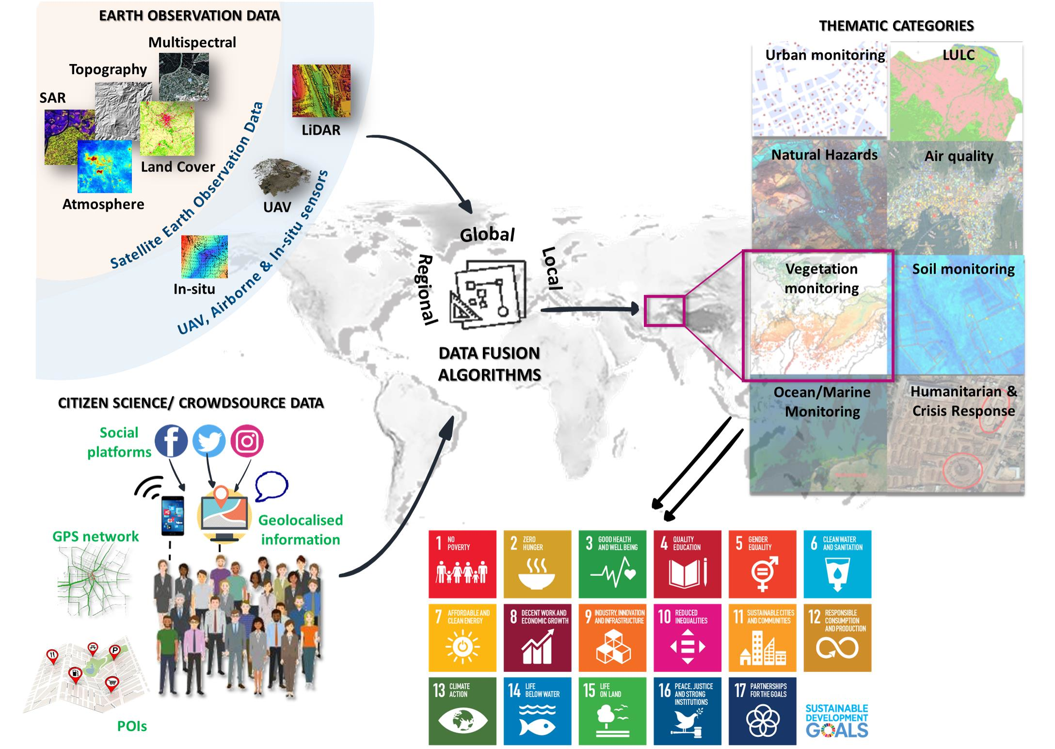
2.1. Earth Observation and Citizen Science Data Proliferation: The “Footprint” of the Digital Age

Two significant landmarks appeared in the 21st century as the ones that can facilitate to better understanding the world’s needs; the provision of global-scale, open-accessed Satellite data and Web 2.0, which has culminated in the rise of crowdsourcing and the citizens as a sensor information [13,14,15]. Recent solutions have placed EO in the highest position of the data landscape as a cost-efficient solution that could provide more accurate estimations on the future dynamics of the human-Earth system [16]. Under this frame, various international organisations such as the Committee on Earth Observation Satellites (CEOS), the Global Climate Observing System (GCOS), and the Group on Earth Observations (GEO) were established to design and further certify the scalable and interoperable nature of EO systems [17]. In 2016, the European Space Agency (ESA) initiated the Earth Observation for Sustainable Development (EO4SD) program to explore the existed EO-missions in numerous applications, such as agriculture and rural-urban development, water resource management, climate resilience and natural hazards reduction. With the combinations of the EO and ancillary data from static sensors, model simulations’ outputs, and others, now we shall claim that we are in the most convenient position to monitor our planet [18] accurately. Opposing this statement, even if such a tremendous amount of information surrounds us, it usually lacks semantic meaning. Traditional methods of visual inspection and photo interpretation are still performed for the acquisition of reference data and therefore described among researchers as a bottleneck and an unsustainable way to extract meaningful outcomes for the heterogeneous, complex, imperfect big-EO data [19].
Overcoming this obstacle, citizens have proven a meaningful addition to the environmental sciences as they are capable of creating content in various ways, i.e., through image interpretation, collection of in situ data, and social media [20]. Mialhe et al. [21] declared that the VGI derived from citizens and stakeholders could reveal rich and complex information of the local environment and its change through time; a hard to gain knowledge by other data forms or experts. Capitalising on the pioneering work of Goodchild [12,22], in the last two decades, a significant amount of initiatives and projects incorporated the VGI as a valuable source of information. Indicative examples are the EU-funded projects of hackAIR [23], SCENT [24], the ARGOMARINE [25], E2mC [26], and GROW Observatory [27]. The hackAir project (www.hackair.eu; accessed on 28 February 2022) has developed an air quality data warehouse, where large communities of citizens can provide air quality measurements with easy deployment of low-cost sensors. Subsequently, the air quality conditions are further expanded using a combination of official data and sky-depicting images. SCENT (https://scent-project.eu/; accessed on 28 February 2022) demonstrated a collaborative citizen engagement tool, enabling the land-use/land-cover change (LULCC) data collection. Semi-automated and machine learning classification methods were utilised to evaluate the collected observations and extract semantic descriptions of the ground-level images. An innovative contribution of CS to the improved monitoring of marine water quality is offered by the ARGOMARINE mobile application (http://www.argomarine.eu/; accessed on 28 February 2022), allowing citizens to provide notifications of detected oil spills, assisting on the efficient and responsive mitigation actions. E2mC (http://www.e2mc-project.eu/; accessed on 28 February 2022) aims to expand the Emergency Management Service (EMS) of Copernicus, exploiting the beneficial contribution of social media data to the rapid evaluation of the satellite-based map products and subsequent reduction of timely effort of producing reliable information. One of the fundamental projects of CS is the GROW observatory (https://growobservatory.org/; accessed on 28 February 2022), which demonstrated a complete “Citizen Observatory”, resulting in a targeted audience of different stakeholders (i.e., smallholders, community groups, etc.), creating soil and LULC monitoring system.
In addition to the broad applicability of volunteer crowdsourcing in several domains, still, it is essential to encapsulate the citizen role, not only as a data collector but as a contributor and collaborator to a citizen science project [28]. Many terms have appeared across the literature [15,20,29], with a will to describe the crowdsource data, based on the role of citizen within the project, with the “passive and active crowdsourcing” [30] to be met in the majority of studies. Former studies defined the role of citizen in EO depending on the nature of the crowdsourcing task [31] and the technological equipment that was used, identifying two additional types of crowdsourcing, the "Mobile Crowdsourcing" [32], where citizens act as moving sensors [33,34], and the social media. The recent growing number of publications in social media testified the tendency of the research community to invest in passive (or opportunistic) crowdsourcing and the semi-autonomous or autonomous information extraction [35]. An example of opportunistic sensing is the pools of geotagged photos that rapidly increase, declaring almost 2 million public photographs uploaded to Flickr, and around 58 million images per day to Instagram [36]. Nevertheless, the inclusion of such vast volumes of EO and CS data generates significant difficulties in the production of meaningful outcomes to decision-makers, related to the Big Data characteristics (i.e., denoted as the 5Vs: Volume, Variety, Velocity, Veracity and Value) [19].

2.2. Assimilating Data from Space and Crowd

Historically in remote sensing, the four dimensions of spatial, temporal, spectral, and radiometric resolution are denoted as the cornerstones of EO [37], and thus different acquisition sources have been coupled and jointly analysed by the data fusion techniques to achieve richer descriptions of them [38]. Data fusion, sensor fusion, information fusion, or simply fusion is utilised as a powerful way to assimilate various sources of information and therefore achieve a better outcome [38]. White [39] could be considered as one of the first researchers that attempted to define the DF as, the association, correlation, and combination of data from single or multiple sources to achieve refined spatial, temporal and thematic estimates, and evaluate their significance. Different taxonomy views and architectural schemes have been used to effectively describe data associations. Meng et al. [19] and Salcedo-Sanz et al. [18] examined the main building blocks of DF. In particular, these blocks exploit (i) the diverse data sources from different positions and moments, (ii) the operational processing that refines (or transforms) the pre-described data, to be ingested on the DF model, and (iii) the purpose that defines the model that is implemented to gain improved information with fewer errors. In the second article, post-processing was mentioned as an additional methodological step that is applied to update model’s outcomes and enhance their accuracy. From a broader view, several methods were designed, attempting to unify the terminologies that have been used and better understand such a complex system as data fusion is. However, a dedicated analysis of the DF models exceeds the scope of this study, and thus Figure 1 aims to report the most wide-spreading architectures and their corresponding divisions.
In Remote Sensing (RS), DF is usually defined by the level at which the EO-data is at hand, and is categorised into pixel, feature, and decision. Starting with the first raw/pixel, it refers to procedures that utilise different modalities with a will to generate a new enhanced modality. This includes applications of pan-sharpening, the super-resolution and reconstruction of a 3D model. The feature DF level aims to augment the initial set of observations, as linear or spatial transformations of the initial data, and finally, the last level represents the decision DF, where data represent a specific decision (e.g., LC class, or the presence/absence of an event), and is combined with additional layers to increase the robustness of the prior decision. Schmitt and Zhu [41] presented a state-of-the-art (StoA) review in data fusion techniques and algorithms for Remote Sensing and claimed that among the most sophisticated fusion tasks, the real challenge is to combine significantly heterogeneous data. The EO-DF with the crowdsourcing data appeared to be of great interest. An obvious benefit is the large magnitude of available data, the fact that CS offers timely and near (real-time) monitoring and analysis, as well as its availability in online publicly accessed repositories [35]. There is a growing interest in applications that use CS data from social media, crowdsourced open access data repositories (e.g., OSM, GeoWiki, Zooniverse, etc.), geotagged shared photographs (e.g., Picasa, Flickr, etc.), web scrapers and many more [42,43]. Fritz et al. [20] listed a remarkable number of CS projects in different disciplines of RS, including air quality, collection of environmental data, natural hazards, land-use/land-cover, and humanitarian and crisis response. On the contrary, CS data has been criticised due to its intense noisy nature, thematic inconsistency, and lack of usability. Various studies tried to solve these challenges and enhance the performance and credibility of CS data, using noise-tolerance classification algorithms [44], rule-based thresholds and methods that eliminate errors and biases in the training data [45], with significant results [46]. Inevitably, citizens have proven a viable data gathering tool, able to cover the limited quantity of training data, an issue that is often the cause for poor model’s performance [45].

3. Methodological Framework

In this analysis, a systematic scoping review is presented, following the steps of Daudt et al.’s [47] and Arksey and O’Malley [48], to explore the current state of knowledge regarding the pre-determined research questions [49,50]. Data fusion algorithms, data streams and tools are examined with a focus on research works that assimilated data from Crowd and EO (satellite, aerial and in situ) sensors. A priori research protocol was designed, based on the proposed steps of Arksey and O’ Malley [48], and Peters et al. [51].

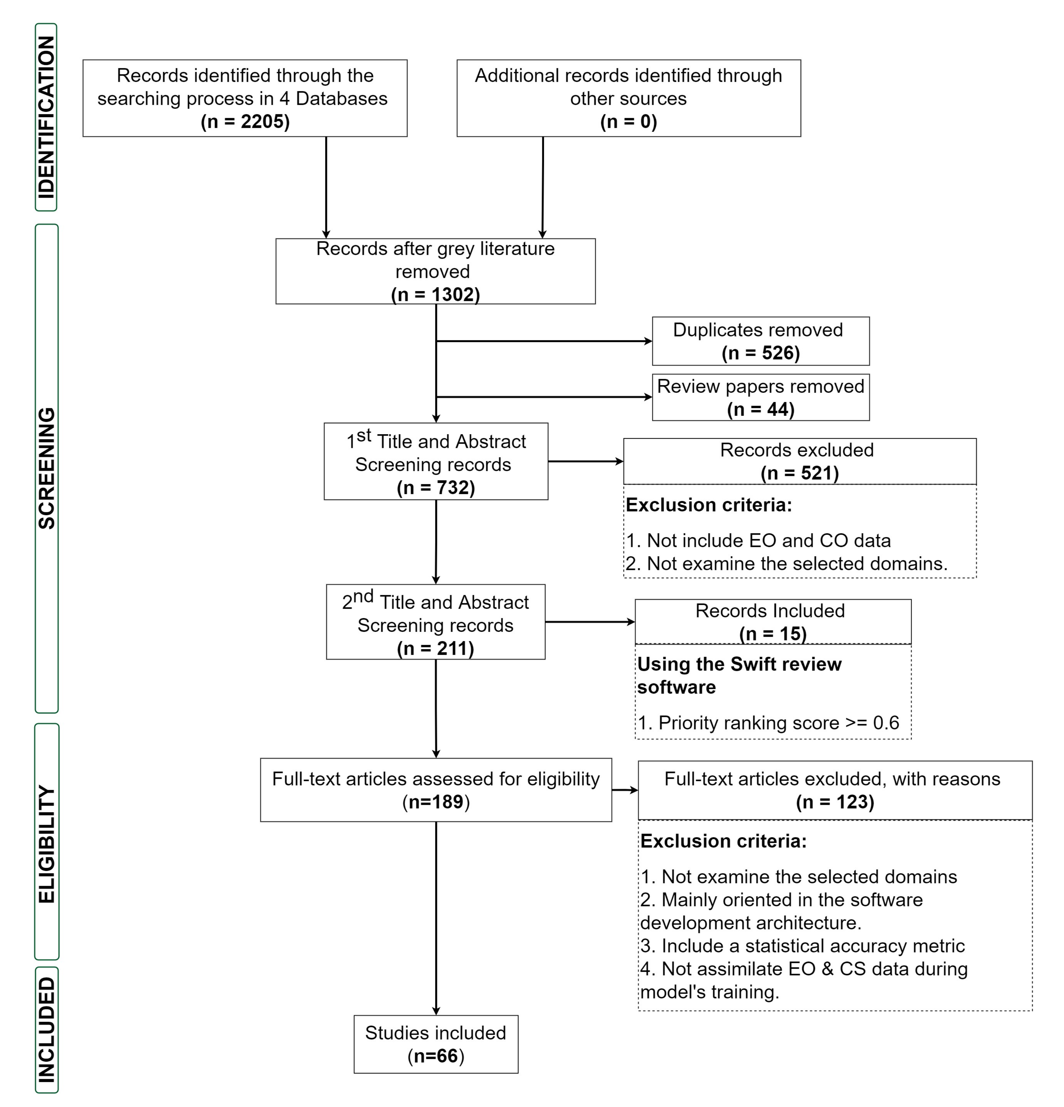
3.1. Search and Selection Strategy

We initiated this analysis, searching English-language based peer-reviewed journals in the four electronic literature databases of Scopus, Google Scholar, ScienceDirect, and Taylor and Francis. To implement this preliminary criterion we excluded any manuscript, characterised as “grey literature” including conference papers, presentations, book chapters, commentary, extended abstracts, preprints, etc. The searching period is between 1 January 2015 and 31 December 2020, following the work of Saralioglu and Gungor [52] and Fritz et al. [20] that indicated an increase in the number of published articles that combine both EO and CS data. Boolean operators combining multiple keywords relevant to the research topic are depicted in Table 1 and were queried in the aforementioned databases. All results were uploaded to Mendeley software to remove any duplicates. Subsequently, visual inspection was performed to exclude any remaining grey literature that was not automatically obstructed.
A double and two-level screening (abstract screening and full-text screening) methods were adopted using an iterative review team and the systematic review software, Swift-Review [53]. This software is built on the latent Dirichlet allocation (LDA) model, where few pre-trained data are manually labelled (i.e., as “relevant” or “non-relevant”) and are used to predict the conditional probability of each document as “relevant” [54]. As a result, the most “representative” documents get the highest scores and are presented at the top of the list. The double screening procedure consists of two stages with the first including triaging the publications in “Relevant/Non-Relevant” and thus performing the priority ranking, and the second to evaluate the predicted ranking scores, denoting the threshold of relevance. This method included screening the title and abstract of each publication, where a 50/50 ratio of training and test sample was randomly selected, ensuring the objectivity of the data sample. An evaluation of the model’s results was conducted, investigating the quality of the ranking scores against authors’ criterion of “Inclusion/Exclusion” (Inc/Exc), leveraging the visual-inspection process, the confusion matrix post-processing analysis and the sensitivity evaluation metric, formulated through the following equation. The validation process was initiated, denoting as “Relevant” the corpus of a prioritisation ranking score of 0.6 or higher. Subsequently, we obtained the proportions of true positive (TP), and false-positive (FP) and synthesised the sensitivity score. The dataset was updated including the validated “Relevant” articles and the remaining articles, which were denoted as “included” during the first abstract screening process. Thereafter, the final dataset was confirmed, ascertaining the corpus selection efficiency through the full-text screening procedure. The selection procedure and the adoption of the selection criteria are presented in the section below.
S e n s i t i v i t y = T P T P + F P ,

3.2. Selection Criteria

A research team of 3 expert reviewers (one in Earth Observation, one in Citizen Science, and one in Artificial Intelligence and data assimilation algorithms) was formed, who applied the same post-hoc Inc/Exc criteria, were given a deadline of 2 months after the initiation of this process. The Inc/Exc criteria were defined at the beginning and prior to the selection process, ensuring a reduction of bias and the thematic consistency of this analysis [55]. All the reviewers had to justify the Inc/Exc of each examined publication and a consensus had to be achieved for the final inclusion of each document.
Inclusion Criteria:
  • Publications must be Peer-reviewed scientific journals, written in the English language.
  • Peer-reviewed articles have to be published between 2015 and 2020.
  • Publications encompass data from satellite, aerial or in situ sensors with crowdsourced data.
  • Studies that focused on land terrestrial applications, addressing the following research domains, among the different thematic categories presented in [20].
    (a)
    Land Use/Land Cover (LULC)
    (b)
    Natural Hazards
    (c)
    Soil moisture
    (d)
    Urban monitoring
    (e)
    Vegetation monitoring
    (f)
    Ocean/marine monitoring
    (g)
    Humanitarian and crisis response
    (h)
    Air monitoring
  • Articles may validate their proposed method using a statistical accuracy metric.
Exclusion Criteria:
  • The literature review publications.
  • Studies that solely use EO or CS data are excluded from the review.
  • Any publication related to the investigation of extra-terrestrial environments.
  • Articles that oriented their research on platforms visualising data, without applying data fusion methods among EO and CS data.
  • Exclusion of studies that did not assimilate both EO and CS data during the training phase of the presented algorithm. Articles, where one of the two data types is utilized for validation purposes and therefore did not contribute to the model’s prediction, are excluded for further investigation.

3.3. Charting the Data: Transformation, Analysis and Interpretation

The literature was charted after a common agreement of the reviewing team and is presented in the following sections, illustrating the processes that attempted to combine the disparate information [48].

3.3.1. General Categories

In this category, titles and abstracts were explored along key characteristics such as literature sources, year of publication, thematic categories, and mapping scale. Regarding the spatial extent, this (i.e., the mapping scale) was categorised as local, regional and global (Table 2), following Tobler’s rule [56], which associates the mapping scale with a spatial resolution of RS images. In cases of multiple EO data, at diverse spatial resolutions, the category was determined according to data with the finest spatial resolution, denoting as the minimum size of an area that can be detected, or to authors’ pre-defined minimum mapping unit (MMU).

3.3.2. Applications Assimilating EO and CS Data

The literature is organised with respect to the general thematic categories that are already presented in Section 3.2, and are subsequently mapped to the main applications of interest in these particular domains.

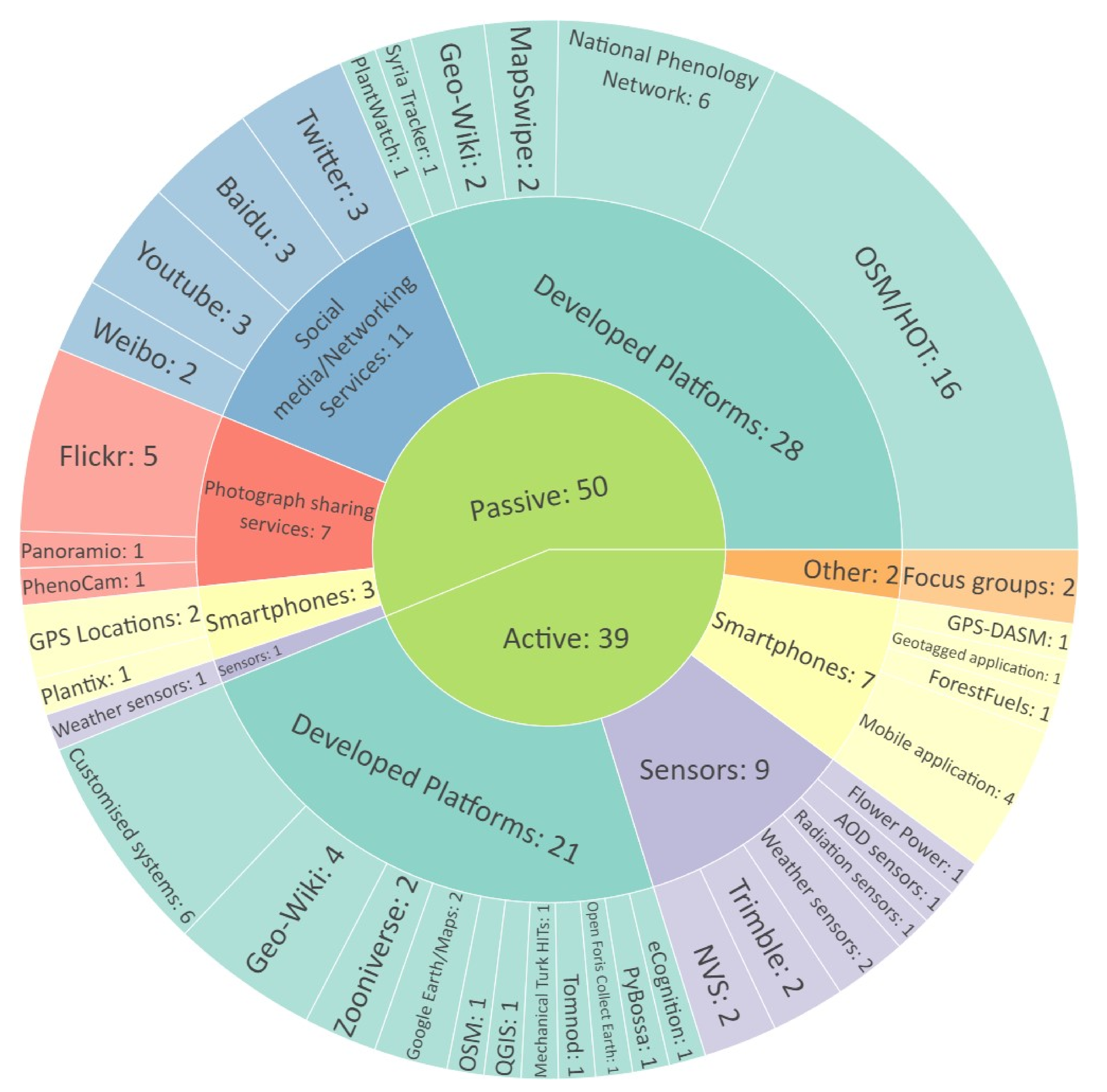
3.4. Exploitation of EO Data and Crowdsource Data Gathering Tools

The selected papers were organised into two distinct categories: In the EO data section, the environmental/climatic and non-environmental variables are examined as well as the satellite EO platforms and datasets that appeared across the selected cases. Furthermore, crowdsourced data and tools are classified with respect to citizens’ participation type, denoted as “active” or “passive” [5,8], or as Foody et al. [11] stated “participatory sensing” and “opportunistic sensing”. Participatory sensing will include articles that indicate the actual involvement of citizens in the data collection and the design of testbed environments [30], whereas opportunistic sensing incorporates publications that describe automated processes of crowdsourced data extraction from open-access tools and platforms. In both cases, the selected corpus will be organised with respect to the technological equipment that was used, considering the following classes.
i
Social media/networking services (SM): Including commercial platforms, developed for sharing social information content (text, sound, image, and video).
ii
Photograph sharing services (PH): Web services, sharing geotagged photos.
iii
Sensors (S): Low-cost sensors, such as magnetometers, accelerometers, etc.
iv
Smartphones (SP): Mobile crowd-sensing (MCS) [15] devices including their functionalities of GPS, or geotagged photos, etc.
v
Developed Platforms (DP): Open access crowdsourcing platforms, such as Geo-Wiki, Tomnod [57], Humanitarian Open Street Map, and customised solutions.
vi
Other: Referring to studies with an absence of technological equipment. An example of this case is presented in Mialhe et al. [21], where transparent plastic films were used to define the land use categories.

3.5. CS Data Uncertainties and Methods for Data Curation

Despite the research advances, data curation and lack of trust in crowdsourced data still remain a challenge. This category aims to qualitatively describe the identified challenges and the methods that were utilised to validate and reduce any discrepancies in CS data. Proposed indicators and methods are described according to the step where the validation has occurred, denoted as “ex-ante” and “ex-post”, and the relevant crowdsourcing task [57].Three CS tasks of classification, digitisation and conflation [57], and related classification problems (e.g., multiclass, or binary) will be discussed and associated with the level of spatial and cognitive complexity of CS data retrieval.

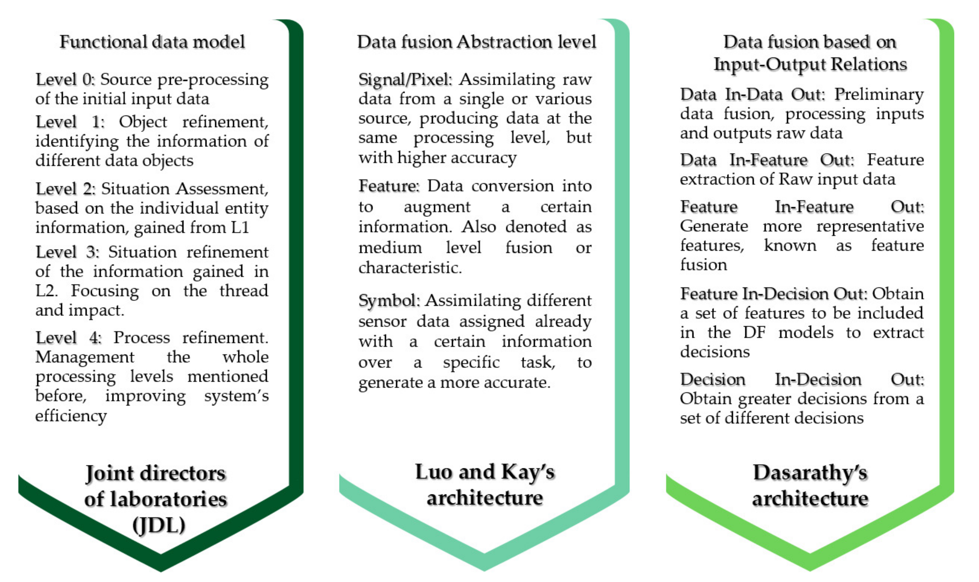
3.5.1. Data Fusion Models and Evaluation Approaches

The definition of the selected corpus with a single taxonomy seems quite challenging, if not impossible [18]. For this scoping review, a hybrid data fusion schema is explored, mapping the RS data fusion terms (i) pixel/data, (ii) feature, (iii) decision [58,59] to the following four levels of abstraction [40] (i) Low-level fusion, (ii) Medium-level fusion, (iii) High-level fusion and (iv) Multiple-level fusion. Articles that integrate data types (e.g., images, texts, etc.) at different DF levels are included in the fourth abstraction level. Note that any fusion method implemented in the stages of data preparation or model evaluation, or that refers to EO or CS data solely, is excluded. Methods are categorised as statistical, mechanistic, and data-driven with the sub-categories of Artificial intelligence, Ensemble, and Fuzzy Association, also analysing the quality assessment methods and evaluation metrics that were applied.

3.5.2. From Data to Information, towards Decision Making

Charted data are analysed using both descriptive and quantitative approaches [60]. In the descriptive analysis, a network visualisation map was created based on the selected literature and the VOSviewer open-access software [61]. N-clusters and linked relationships were generated according to the level of relevance between the predicted terms and frequency of occurrence. The terms are presented in a weighted form, indicating the most frequent terms with greater weights. The predicted terms in the network graph were evaluated according to the terms’ relevance and the scope of this analysis. Generic keywords or keywords irrelevant to EO, Citizen Science/Crowdsourcing and Data fusion/Machine learning domains were avoided. In the quantitative analysis, graphical representations were designed, aiming to give intuitive messages regarding the examined research questions; the web-based software Datawrapper and the Python libraries of Pandas and Plotly were used.

3.6. Bias Control

In order to reduce bias in this scoping review, Lapierre et al.’s [62] guidelines were followed that aimed to control two types of bias, the publication bias and the ratter bias [63]. Regarding the first, the authors ensured the provision of research outcomes with transparency, using four electronic literature databases (Scopus, Google Scholar, ScienceDirect, and Taylor and Francis), in which only peer-reviewed journals were included, avoiding any restriction related to journals’ level of impact. Continuing, the ratter bias was mitigated following an iterative review process of the predefined scope by a balanced research team of 3 reviewers. On top of this, the systematic review software Swift-Review has solved the rare cases of disagreement between the reviewers.

4. Results

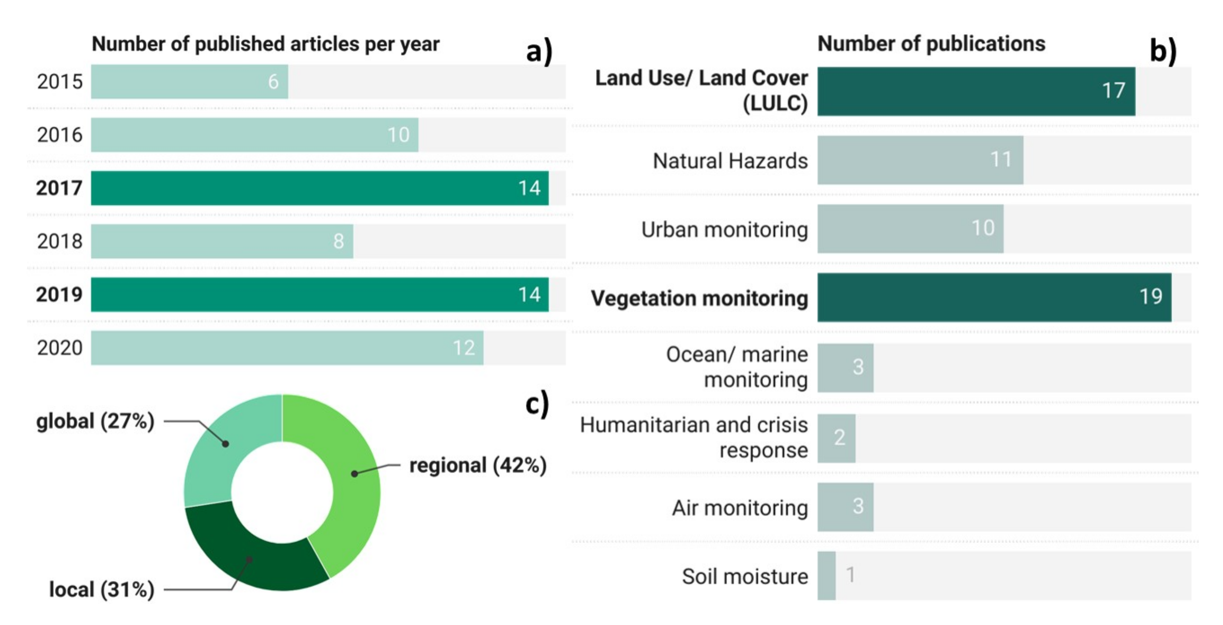
4.1. General Overview of Process and Findings

The association of RS and CS data was initially identified in 2205 published articles, retrieved by the four electronic databases, referring to the period of 1 January 2015 and 31 December 2020. The articles were further reduced to 732 after the exclusion of the grey literature and duplicate records. During the double abstract-screening process, 15 additional publications were found relevant, following the prioritisation modelling and the statistical evaluation. The ranking scores of the examined literature varied from 0.094 to 0.921, from which approximately 90% of the “Relevant” documents were listed at 50% of the top-ranked documents. Relevant documents were identified in 70% of the top-ranked data, (Figure 2). The statistical findings resulting from the prioritization modelling were evaluated with a threshold of relevance (i.e., ToR = 0.6), using the confusion matrix method and the sensitivity evaluation metric [64]. Note that ToR was empirically defined based on the authors’ observations on the selected literature. The sensitivity score of 80% was estimated exploiting titles-abstracts only and thus seemed acceptable for further processing, (Table 3).
During the full-text screening, different data fusion algorithms and processes were identified. Such processes have been successfully organised by Bleiholder and Naumann [65] into two categories, i.e., data integration and data assimilation. The first refers to the notion of a unified information system, where data are stored and presented to the user in a unified view, while the second focuses not only on a common data interpretation but on the generation of new real-world objects. In the data assimilation system, information by various sources is harmonised, based on a pre-designed and three-level mapping schema (i.e., transform, remove duplicates, and concise), and integrated into numerical models and algorithms in order to produce a new decision [66]. Considering the above, this scoping review focuses predominately on articles describing the data assimilation models, involving EO and CS data as well as any auxiliary geospatial information. Adhering to the latest criterion, a total of 66 scientific articles were finally selected as they met the eligibility criteria (Figure 3), and are briefly presented in Table A1, Table A2, Table A3, Table A4, Table A5, Table A6, Table A7 and Table A8 of Appendix A.
Analysing the 66 selected articles, a thorough view is formulated based on the general characteristics of the selected documents. Particular attention is given to the peer-reviewed journals, the number of publications addressing the most common thematic categories as described in Section 3.2, the number of published articles on annual basis, and the mapping scale levels, where models were tested.
The majority of the peer-reviewed journals (56%) that are published in the 9 scientific journals are presented in Table 4. A total of 29 articles appeared only once and thus are aggregated under the “Other“ category (44%). The majority of the aforementioned journals focuses on environmental, or climate change ecosystems, whereas the journals ranked in the top four positions (i.e., Remote Sensing|n = 14, ISPRS Journal of Photogrammetry and Remote Sensing|n = 5, Remote Sensing of Environment|n = 4, IEEE Transactions on Geoscience and Remote Sensing|n = 3, and International Journal of Applied Earth Observation and Geoinformation|n = 3) predominately oriented their studies in the RS applications.
Following Fritz et al.’s [20] findings, we examined the articles published between 2015 and 2020 (Figure 4a), and those related to the thematic categories presented in Section 3.2, (Figure 4b). A categorization with respect to the economic status of the selected regions was performed, revealing two maxima in 2017 (n = 14) and 2019 (n = 14), decreasing in the last year of the searching riod. However, continuous high numbers of published articles indicate that the contribution of EO and CS data in the decision-making and management processes is continuing to grow [68]. With respect to the results in Figure 4b, the greatest number of articles refers to the categories of Vegetation monitoring (n = 19) and Land Use/Land Cover (n = 17) with a negligible difference among them, whereas the Humanitarian and Crisis Response (n = 2), gained the least attention. Finally, only one article is related to the Soil moisture domain, indicating that the fusion between the EO and CS data for this specific application is still in its infancy [69].
Considering the ratio of articles per mapping scale (Figure 4c), a greater preference is shown in studies with high and medium mapping scales (local|regional|global = 31|42|27%). More intuitive findings regarding this research question are presented in Section 4.3.3. The primary conclusions follow next: First, the tendency to exploit the regional-scale data was an expected result, as data at finer resolution are predominantly not freely distributed. Additionally, we could claim that citizens might feel more engaged with studies at familiar scales or to a phenomenon that directly affects them, revealing a lower interest in global-scale applications. This basic assumption is also evaluated by Tobler’s first law of geography (TFL), which implies a direct and strong relationship between things that are closely located [46]. Recent studies in the quality of the Volunteered Geographic Information (VGI) indicate that volunteers tend to perform the VGI tasks with greater success when they are located in areas close to volunteers’ homes [70]. Yet, continental or even global scale effects of humanitarian or natural disasters are still unknown to the public, or presumably not evident in citizens’ everyday life.
A clustering visualisation network was used, as an alternative to the words’ of cloud method, as it was able to elicit more meaningful results from unknown patterns, containing keywords and phrases that were referred in combinations in most documents. The clustering network graph was generated after several trials, evaluated by authors and displayed in Figure 5. A total of 49 keywords are visualised in eight core clusters, coloured in red, green, blue, light blue, yellow, purple, orange and brown, extracting the main research domains of this paper. Each cluster was structured with nodes closely located to each other and linkages among them, where each node is denoted from the assigned colour that indicates the cluster category, and the relative size, presenting “keyword’s importance” and the frequency of occurrence. Links between the terms indicate the strength of the term and its association with various terms. Therefore, nodes with higher “keyword importance” tend to have higher linkage strength; whereas, the colour of the link is related only to the node’s class.
Viewing the results, we could conclude that keywords with the highest frequencies were “classification/class” (61), “model” (59), “image” (42), “observation” (37), “phenology” (18), “open street map-OSM” (31), “volunteer” (16), “land cover product” (14), and “citizen” (14), revealing the two basic terms of our review, i.e., “Earth Observation” and “Crowdsource/Citizen Science”, and an increased interest to applications related to vegetation species, and their phenological stages, and also to land cover products in rural and urbanized environments. However, in some cases, the Lin-Log/Modularity method was not able to identify similarities in common terms, and thus terms such as “classification” and “class”, or “open street map” and “osm” are revealed in different nodes. To deal with this issue, both keywords’ importance and strengths of links were calculated and are presented in an aggregated form. Moreover, it seems that the highest number of links occurred in the same terms that presented the highest frequencies, a result that was actually expected. In particular, the keywords “model”, “classification”, and “image” revealed 42, 32, and 24 links, associating themselves with almost all terms in the graph. Therefore, we could assume that the majority of approaches addressed a supervised data-driven classification problem, where patterns among features are known, and defined by the reference dataset, collected either by citizen-science data or by experts (scientists or national data). Investigating the clusters depicted in Figure 5, three major groups could be defined, in the left (red), right (green and blue) and upper side of the graph (purple), separating themselves with the largest distances. In these groups, keywords revealed an association with the most referenced thematic categories, i.e., Land Cover/Urban monitoring, Vegetation monitoring, and Climate change. The aforementioned result is also in agreement with the results depicted in Figure 4b.

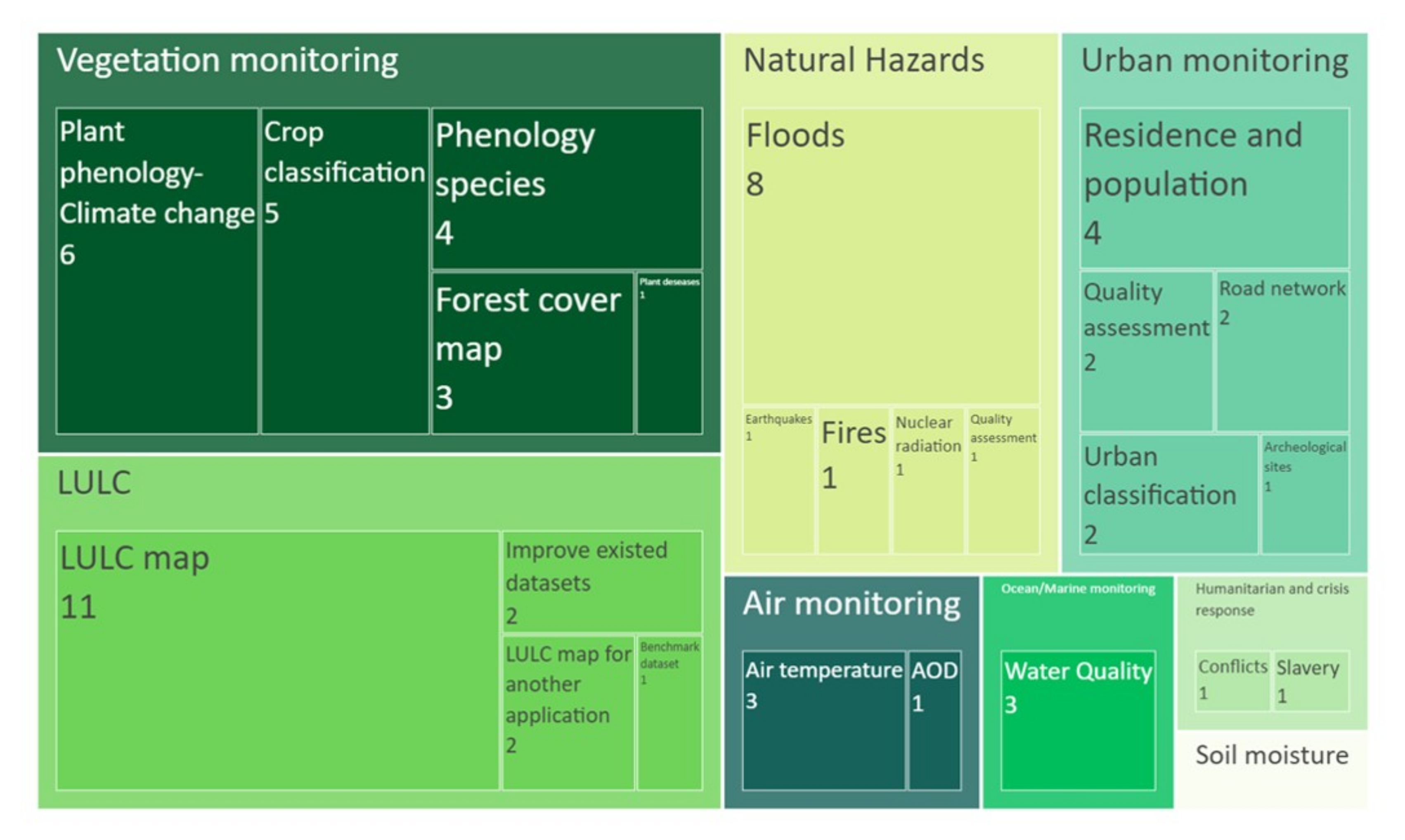
4.2. Applications Assimilating EO and CS Data

In the following sections, a categorisation of the selected literature is done to illustrate the main applications for each examined thematic domain. Figure 6 depicts the share of the applied methodologies, where the RS and crowdsourced data co-existed.

4.2.1. Vegetation Monitoring Applications

Five application types were identified in the Vegetation monitoring domain, including studies that investigated the phenological shifts as a result of climate change (n = 6), the identification of different phenological species along with their properties (n = 4), cropland and forest maps (n = 3&4), and plants with a certain disease (n = 1). The articles in the first category utilised both mechanistic models (n = 2|[71,72]), as well as data-driven approaches (n = 4|[60,73,74,75]) to provide information on either the date of occurrence of a start-end of the season (SOS or EOS) [75] phenophase stages or the transitions of the four stages (i.e., green-up, maturity, senescence, and dormancy) [60]. Xin et al. [75] evaluated the performance of eight different algorithms, six representative rule-based algorithms and 2 machine learning models (i.e., the random forest regression and the neural network) regarding their ability to identify the two phenological phases of SOS, and EOS, as it can be expressed through the MODerate Resolution Imaging Spectrometer (MODIS) Enhanced Vegetation Index (EVI) observations. In four articles (n = 4|[46,76,77,78]), similar approaches were applied focusing on specific vegetation species and the identification of their biophysical characteristics (i.e., tree height, diameter breast height, basal area, stem volume, etc.). In terms of physical models, the Spring Plant Phenology (SPP) models [71] encompass meteorological observations (i.e., temperature, and precipitation), and EO-vegetation data [72] to predict the timing of leaf emergence.
Considering the two categories of crop classification (n = 5|[3,79,80,81,82]) and forest cover map (n = 3|[83,84,85]), most articles attempted to combine the already available LC data and provide updated maps identifying any uncovered areas [83]. Under this frame, multiple datasets were used, i.e., RS land cover datasets [3] and regional or national maps in several countries [85]), EO data at different spatial resolutions (e.g., commercial and open-source satellite and VGI data), auxiliary data (e.g., FAO cropland statistics [84], and sub-national crop area statistics, [82]). A noteworthy study is by Baker et al. [79], which exploited the advantages of citizen science for the identification of urban greening areas at a finer scale, denoted as domestic gardens. In this study, a participatory citizen campaign was organised along with a social media campaign to encourage citizens to participate and provide information related to the garden spaces. One publication [86] exploited the computer vision models (i.e., object detection) and Unmanned Aerial Vehicle (UAV) RGB images, proposing a disease diagnosis tool that could recognise changes in plants’ foliage (i.e., symptoms), at a sub-leaf level.

4.2.2. Land Use/Land Cover Applications

Studies in this category revealed a preference for applications aimed at providing accurate LULC classification maps (n = 11|[21,44,45,87,88,89,90,91,92,93,94]), with an increased interest for such maps in middle and low-income countries. Fonte et al. [94] proposed an automated method of successively filtering the OSM data, avoiding the procedure of the manual verification of their quality, and producing accurate land cover maps. The OSM2LULC_4T software package seemed capable of successfully converting the OSM data to land cover observations. Uncertainty in the land cover data and the CS data quality (n = 2|[95,96]), along with traditional time-consuming procedures, activated researchers to investigate new methods that could overcome class label noise, or “attribute noise” [91]. Factors of noise origination [45] are the presence of dense clouds over the scene acquired by optical sensors, semantic gaps in LULC categories [87] and discrepancies in thematic consistency and spatial accuracy [95,96]. Furthermore, two articles [2,97] introduced a different annotation scheme, called the Local Climate Zones (LCZ), used to better describe the local climate conditions in urban and rural landscapes [2]. Finally, Li et al. [64] generated a large-scale benchmark dataset for deep learning applications, exploiting the effective integration of VHR RS and CS data. Still, the existence of such datasets is limited, preventing RS experts from improving their models or developing new algorithms. Therefore, fabricating RS benchmark datasets still seems challenging, as RS images consist of complex objects, representing more than one land cover type (e.g., mixed pixels at RS images with coarser resolutions), and are affected by the corresponding factors illustrated before [64].

4.2.3. Natural Hazards Applications

The most articles (n = 8) under the natural hazards category revealed an association with flooding episodes. In particular, flood risk mapping was examined in five articles [98,99,100,101,102] with the first two focusing on the estimation of flood extent (i.e., water depth, and water extent), and the last on the flood susceptibility assessment. In the first category, 1 and 2D hydrologic/hydraulic models, as well as data assimilation (DA) models (e.g., Kalman filter) were exploited integrating both physical sensors as well as the WeSenseIt crowdsourcing smartphone application. On the contrary, univariate or multivariate statistical methods, as well as probabilistic models (e.g., Weights of Evidence [102]) were applied for the estimation of the flood susceptibility rate over an area. In these articles, various factors (e.g., environmental and meteorological factors) and enablers, including web search engines [100], photo-sharing platforms (i.e., Flickr site) [102] and participatory campaigns [101] revealed their potential contribution to monitor flood occurrences, and to generate up-to-date and accurate datasets of flooded areas. Furthermore, the study by Ahmad et al. presented an automated flood detection system, called JORD [103], which is the first system that collects, analyses, and combines data from multi-modal sources (i.e., text, images, videos from social media platforms) and associates them with RS-based data in real-time, in order to give estimations of areas that were affected by a disaster event. Panteras and Cervone [104] explored the level of significance of crowdsourced geotagged photos in flood detection methods and thus gave an alternative in cases where the EO data are not available. Finally, Olthof and Svacina [105] evaluated the efficiency of various data sources for receiving information on a flood event, such as passive and active satellite sensors, high-resolution DEM, traffic RGB cameras, and crowdsourced geotagged photos. It also investigated associated methods, i.e., rule-based image thresholds, the coherent change detection proposed by Chini et al. [106] and the 1-dimensional flood simulation algorithm, with the intention to provide accurate urban flood maps within the first 4 h of a flood event. Subpixel mixing in optical sensors, the coarse spatial resolution of Sentinel-1 data and the occasional contributions of citizens seemed the main limitations of real-time flood monitoring.
In addition to flooding events, the following three articles, explored the potential contributions of crowdsourced data in cases related to fire, earthquake, and nuclear accident events. The first case presents the benefits of using smartphone applications and a large audience of volunteers to estimate the forest fuel loading in areas close to urban environments (i.e., wildland-urban interface (WUI) areas) [107]. In general, forest fuels have proven structural components in wildfire risk monitoring, and therefore the accurate data collection is of paramount importance [108]. Furthermore, Frank et. al [109] attempted to give conclusions regarding the role of citizen scientists in terms of their contribution in the rapid damage assessment after an earthquake event; in particular, they investigated the noise resistance of two classification methods (i.e., object-based and pixel-based), and the effect of using different labelling methodologies and crowdsourcing tools. Last, Hultquist and Cervone [110] demonstrated -in the Safecast VGI project- the production of a complete footprint for the radiological release over the Fukushima area after the nuclear accident. In this project, 200,000 measurements were collected by citizens and thus associated with reference data collected by in situ sensors.

4.2.4. Urban Monitoring Applications

Articles under this category developed methods and tools to accurately identify objects (e.g., settlements and road networks) in artificial environments. Population estimations were given, as until now the population layers are produced in coarse resolutions exceeding 100 m, and inevitably have a limited representation in small villages and remote regions [111]. Four studies [7,111,112,113], under this category devoted their efforts to assess the spatial patterns of the urbanized environments and additionally provide population maps at a finer resolution. All the aforementioned applications evaluated their methods in low-income countries. Continuing, Zhao et al. [114] and Kaiser et al. [115] introduced us to scalable methods, altering the traditional methods of urban scene classification, where reference data could merely arise by the worldwide Web [115]. Contributors in the first study were the OSM and the social media platform Baidu. The second study tried to overcome the bottleneck of manual generation of training datasets and thus prove the noise resistance of CNN, which could automatically generate annotated images and discriminate object features. Two articles [116,117] explicitly focused on the provision of updated road networks; the first one using GPS data derived by climbers and cyclists, and the second one by taxi drivers. A single publication [118] illustrated the potential of identification of new archaeological areas, leveraging the benefits of participatory sensing, creating synergies between different groups of volunteers, historians, data scientists and heritage managers.

4.2.5. Air Monitoring Applications

After analysing selected studies in the air monitoring domain, two applications may be referenced, the first [119] investigating the benefits of crowdsourcing in the air quality measurements, and the second (n = 3|[97,120,121]) investigating variations in air temperature over urbanized environments. In both cases, low-cost sensors provided an insight into the air temperature and PM2.5 concentrations over the examined areas and therefore attempted to replace the traditional sensors, as they expressed the reference data in the regional-scale models. Venter et. al [120] and Hammerbeng et al. [97] highlighted the potentials of integrating open-source remote sensing and crowdsourced low-cost sensors in air monitoring, and specifically related to the forecasting of heat extremes (i.e., heat waves, and UHI).

4.2.6. Ocean/Marine Monitoring Applications

When it comes to the analysis of aquatic environments, observations focused on factors that affect water quality (n = 3). In particular, Shupe [122] analysed data collected by citizens along with auxiliary data related to land cover patterns (i.e., urban, agricultural, and forestry areas) in order to estimate seasonal variations in water quality and their relation to certain activities, e.g., intense agricultural activities, fertilization, urban expansion, etc. Under the same concept, Thornhill et al. [123] utilised the CS water quality measurements (e.g., N-NO3, P-PO4 and turbidity) of the FreshWater Watch (FWW) project, and established a scalable approach that could facilitate the identification of regional or local key drivers that contribute to the degradation of freshwater quality. Last, the Citclops CS project was introduced by Garaba et al. [124], in which the low-cost and easy to use Forel-Ule colour index (FUI) method was explored along with RS observations of the MERIS multispectral instrument, to collect watercolour measurements, related to pollutant concentrations (e.g., algal density, etc.) [28].

4.2.7. Humanitarian and Crisis Response Applications

Studies by Boyd et al. [125], and Juan and Bank [126] seemed the only cases that attempted to explore the potential of using crowdsourced data for monitoring activities against humanity (e.g., conflicts, and modern slavery). The first study estimated the locations of potential conflicts in Syria using the variables of EO-night lights, and citizens’ reports of casualties. Subsequently, the second case associated the humanitarian crisis of modern slavery with the carbon footprint that results from the chimney brick kilns. Under this study, RS and CS data revealed their critical role in the future termination of modern slavery, achieving the sustainable goals of the United Nations (SDG 8.7: Ending modern slavery and human trafficking, as well as the child labour in all forms) [127], or the so-called “Freedom Dividend”.

4.2.8. Soil Moisture Applications

A single study [69] showcased the potential of using both EO and CS data for the estimation of the soil moisture, a critical variable revealing earth surface processes (e.g., fertility of agricultural fields). In the framework of GROW Citizen’s Observatory (CO) [27] and the open-accessed EO data (e.g., Sentinel-1, Landsat-8, and EU-DEM), three statistical approaches of multivariate linear regression, multivariate regression kriging and co-kriging interpolations were examined, with the first two providing results with greater accuracy. A common limitation for all the deployed methods was the short-range variability of the soil moisture in situ values, which might prevent researchers from exploiting further this particular research domain.

4.3. Exploitation of EO Data and Crowdsource Data Gathering Tools

4.3.1. Environmental/Climatic EO Variables

Among the different predictors observed in the literature, the vast majority of articles used variables that correspond to data on land (e.g., land cover (n = 22), soil and urban surfaces (n = 8), and vegetation (n = 32)), as well as water (n = 6) and air (air quality (n = 2), rainfall (n = 4) and temperature (n = 5)). Articles predominately chose to incorporate predictors related to topographic features resulting from EO-derived digital elevation models (n = 23) and to land cover objects (n = 22), with an equal representation of these datasets. Three publications [7,88,125] exploited the EO-data only as gridded cells (e.g., 30 m × 30 m area coverage) and therefore were characterised as not applicable (N/A), and excluded for this section.
Topography seemed a significant factor in various applications and predominantly in the natural hazards category. Six articles [98,99,100,101,102,107] used the digital elevation/terrain models (DEM/DTM) to extract topographic parameters as predisposing factors, or as the driving force, propagating the channel flow over the gridded floodplain surface [98,99,105]. Indeed, the DEM/DTMs have been associated with several natural hazard cases, such as flood, fire risk assessment, etc., with the majority of them using the first and the second derivatives, i.e., slope angle and curvature, and aspect. Zeng et al. [100] characterised these factors as very good proxies in flood susceptibility models. In Kibirige and Dobos [69] the variables slope, aspect and relief showed the highest level of significance and the Pearson’s correlation to positively exceed the 0.5, compared to the in situ soil moisture values. Additionally, the United States Forest Service (USFS) agency indicated that the aspect, slope position and slope steepness factors greatly influence the frequency and severity of the wildland fire behaviour [128], as the fire is tended to transfer faster in steeper inclinations. Subsequent hydrological variables such as flow direction, flow accumulation and the Compound Topographic Index (CTI) were found in three corresponding studies, i.e., [69,100,101]. The CTI, also known as Topographic Wetness Index (TWI), is a product of upslope areas, flow slope, and geometry functions [129], and therefore a good indicator for runoff risk assessment [130]. Additional environmental studies related to freshwater degradation (n = 1|[123]), road trace identification (n = 1|[116]), urban LC (n = 1|[90]) and forest plantations mapping (n = 1|[81]) were chosen to exploit the above topographic indicators. A noteworthy case was found in Venter et al. [120], in which both DTM and the Digital Surface Model (DSM) were produced from LiDAR airborne laser scanning (ALS) mission, in order to extract the vegetation canopy height model (CHM), and additional variables corresponding to terrain’s ruggedness. The CHM was calculated by subtracting the DTM from the DSM layers. Consequently, morphological metrics of sky view factor (SVF) resulting from hillshade, mean object height, fractional cover, and neighbourhood heterogeneity in object height were used to investigate the microscale temperature effects in urban canopies.
LULC maps were explored by many cases, mostly identified in the Vegetation monitoring articles (n = 12), where information of forested and cultivated areas as well as different vegetation species (e.g., deciduous forests, shrubs, etc.), was retrieved (n = 6). Multiple LULC data, varying in space (e.g., spatial resolution ranging from 30 to 1000 m) and time (e.g., reference year of production ranging from 2000 to 2018) were fused with the intention to produce an accurate global vegetation map and be in accordance with the statistical findings provided by the Food and Agriculture Organisation of the United States (FAO) and national authorities. Schepaschenko et al. [83,84] claimed that hybrid results are of paramount importance, as so far, the intense pressure in forests arising from anthropogenic and natural disturbances, produce uncertainties and large disagreements between the different products. Indeed, global forest models (e.g., G4M) [131], as well as economic, biophysical, and climatic models e.g., GTAP, IMAGE, GLOBIOM, IMPACT [132], have significant differences in terms of their outputs. The same concept was applied by Fritz et al. [3], and Gengler and Bogaert [80] in the production of cropland maps. An exception to the above is Hansen’s global forest cover map, indicated as the most accurate forest map that has been produced so far [85]. Table 5 illustrates the LULC and forest/cropland maps found in the literature. It seems that most of the products are referenced mainly in four articles [83,84,85,96]. Two articles [74,75] exploited the annual vegetation dynamics of MODIS data (i.e., MCD12Q2) to identify the different phenophase stages (e.g., Start of Season or End of Season), expressed as date of the year-DOY.
Furthermore, the LULC products were identified also in the flood susceptibility cases (n = 2), where the LC vegetation classes were proven to have a negative association with flood events [100] or to correspond with the surface roughness properties of the floodplain, with which the Quasi-2D models propagate the flow. This different classification schema over the initial land use categories is denoted as Manning’s roughness coefficient [98]. The second LULC classification schema was developed by the World Urban Database and Access Portal Tools (WUDAPT) and adopted by [2,97,136], in which the urban areas are denoted with 17-LCZ typologies, presenting different micro-climatic conditions. More information on the LCZ classification schema are available in Steward and Oke [137]. Finally, LULC was used to reveal information regarding the land cover/urban objects (e.g., [95,96,112]), and specifically considering the effect of the agriculture activities on water quality [122,123], or the signal loss due to dense vegetation presence [116].
EO spectral indices are important indicators, present in most examined categories, except for the Humanitarian and Crisis Response, and Ocean and Marine monitoring applications. Table 6 shows a preference in Vegetation indices (11/18 total number of identified indices), and especially (n = 12) in the Normalised Difference Vegetation Index (NDVI). Maximum NDVI images per annum were obtained in three articles [45,90,91] to eliminate cloud contamination over the scenes and ameliorate any seasonal and inter-annual fluctuations [138]. NDVI was not restricted only to LULC studies but was also used to detect vegetation species (e.g., invasive buffelgrass [78] and urban orchards [46]), and fuel loads [107], as it can capture variations in chlorophyll absorption patterns of plants, even in cases of understory vegetation (e.g., shrubs, grass), where the reflectance response in Near InfraRed (NIR) is lower. Continuing, the Enhanced Vegetation Index (EVI) was present mostly in time-series models (n = 4), identifying the seasonal disparities in deciduous forests. An interesting method was Delbart’s et al. [73], where the Normalised Difference Water Index (NDWI) was exploited for the green-up estimation date, as an effective solution to avoid false detection due to snowmelt.
Two studies produced multiple vegetation indices calculated by Very High Resolution (VHR) data of the RapidEye satellite [107] and the High-Resolution True-colour Aerial Imagery (TAI) of Getmapping [139], with the latest to leverage on pixel’s colour intensity in visible red and green. Apparently, in land cover classification studies, additional indices are incorporated, distinguishing the impervious surfaces and bare soil lands. Paradigms are the most known (a) Normalised Difference Build-Up Index (NDBI), and the newer indices of (b) built-up index (BuEI), (c) soil index (SoEI), (d) bare soil index (BSI), and (e) index-based built-up index (IBI). Eventually, the Modified Normalised Difference Water Index (MNDWI) seemed to be preferrable compared to the NDWI, when the extraction of water areas is requested, as it is able to suppress the reflectance response of vegetation and built-up areas, and thus to perform better in water detection [102,104]. Therefore, when data from multiple satellite sensors are used, the pre-processing technique of atmospheric correction (e.g., dark subtraction) was applied [88,102,107] in order to avoid inconsistencies related to the sensor’s viewing angle and the different illumination conditions.
Non-invasive technologies and applications on air and water degradation monitoring were leveraged by a hybrid schema of ground- and satellite-based predictors to monitor areas of increased air pollutants concentrations (e.g., PM2.5) or to illustrate variations in microclimatic temperatures [153]. Investigating studies in the first, Ford et al. [119] explored the air quality-related product of Aerosol Optical Depth (AOD) derived by in situ sensors (i.e., AERONET sites), low-cost crowdsourced sensors and the satellite AOD products from MODIS (Aqua and Terra satellite platforms) to reveal the PM2.5 concentrations over northern Colorado. Furthermore, the air temperature was directly measured by in situ meteorological stations [121] and gridded interpolated data (i.e., Daymet and PRISM) [71], or indirectly by using satellite measurements of land surface temperature (LST) [120] as a proxy for the near-surface air temperature (Tair) measurements. Precipitation and water level measurements play an important role in flood risk assessment cases (n = 3|[99,100,101]). Additionally, Walles et al. [78] used precipitation data to reveal correlations with the buffelgrass presence, claiming a faster response to water than native plants, breaking the dormancy phenophase level. In these cases, the precipitation layer was derived from gridded data of the “Parameter-elevation Regressions on Independent Slopes Model” (PRISM) and the static physical rainfall or water level sensors. Finally, the Forel-Ule colour index (FUI) scale was introduced by Garaba et. al [124] as a method to distinguish the watercolours and illustrate primary findings regarding the concentrations of water masses. As a consequence, associations with factors related to water quality such as turbidity, coloured dissolved organic matter (CDOM, also called Gelbstoff), inorganic suspended particulate material (SPM), as well as chlorophyll-a (chl-a), can be achieved [124].

4.3.2. Non-Environmental EO Variables

Although the environmental variables are presented predominantly in this scoping review (n = 57/61), four articles incorporated non-environmental variables, Table 7. Gueguen et al. [111] and Herfort et al. [7] utilised human settlements and urban footprint datasets (e.g., High-Resolution Settlement Layer (HRSL), Global Urban Footprint (GUF), etc.) along with population density layers, in order to produce population layers at a finer scale. So far, existing population layers are created in conjunction with ancillary data such as road networks, census data at coarse resolutions ranging from 100 m to 1 km. This raises awareness, especially in developing countries, where road networks are not well recorded, leading to incomplete or innacurate information. Juan and Bank [126] utilised the annual nightlight emissions retrieved by the Defense Meteorological Satellite Program’s Operational Linescan System (DMS-OLS) as an indicator to map electrified regions over Syria that were assumed to be less prone to reveal conflicts and human losses. Eventually, radiological data retrieved by ground stations are exploited by [110], investigating the spatial expansion of nuclear radiation over the Fukushima region, as well as the spots of the highest risk for citizens.

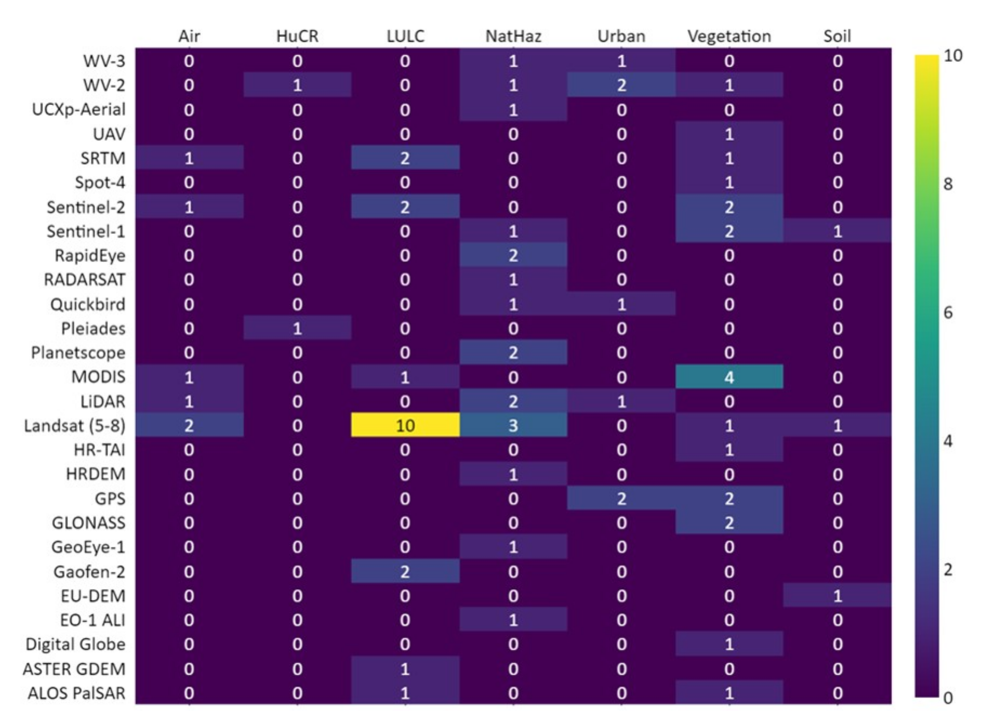
4.3.3. Satellite Data and Sensors Utilised in Data Fusion Applications

Satellite EO data were the main data source across all thematic categories, with only two articles considering data obtained from drones (n = 2| UCXp-Aerial [109] and HR TAI [79]). In Figure 7 the vast majority of articles leveraged optical and multispectral sensors except for seven articles, where SAR data (i.e., ALOS PalSAR and Sentinel-1) [81,91], LiDAR 3D point measurements [118], and combined signals of Navstar GPS and Russian GLONASS Global Navigation Positioning Systems (GNSS) [77,116,117,154] were used. Landsat multispectral sensors (e.g., 5 TM, 7 ETM, or 8 OLI) were exploited in 16 articles (LULC = 10; Air monitoring = 2; Natural Hazards = 3; Vegetation monitoring = 1), with the Landsat-8 OLI dominating among the others. The searching period itself is related to this as well as the “scan line corrector off” (SLC-off) of Landsat-7 ETM+ which drastically decreased its usability [45]. Among different application fields, Landsat data was used to derive spectral indices (e.g., NDVI = 8| [45,69,81,90,91,92,100,120]; IBI = [120]; LST = [120]; NDBI = 2|[90,92]; MNDWI = 3|[90,102,104]; BuEI = [90]; SoEI = [90]), as well as to generate LULC maps (n = 7| [2,21,89,97,122,123,136]). Multispectral satellites, described by similar spatiospectral characteristics, such as Sentinel-2 (10 m), and Earth Observation-1 Advanced Land Imager (EO-1 ALI, 25 m) were used as alternatives by five articles [81,89,94,104,120].
Satellite sensors at lower spatial resolutions (≤250 m), such as MODIS appeared in regional or global scale studies (n = 5), providing “analysis-ready data”(ARD) of surface reflectance, phenology related indices such as EVI [60,93], NDVI [78], LC (NLCD2011) [60], and the Aerosol Optical Thickness/Depth (AOT/AOD) measurements at 550 nm [119] (MYD04/MOD04). Examples of the MODIS datasets that were used across the literature are the Nadir Bidirectional Reflectance Distribution Function-Adjusted Reflectance (NBAR) (MCD43A4, Version 005) [72], 8-day surface reflectance data at 500 m spatial resolution (MOD09A1 Version 006), the twice-daily surface reflectance data (MOD09GA and MYD09GA, Version 006) [60], the Vegetation Dynamics dataset (MCD12Q2 Version 006) and the Annual Land Cover Type at 500 m (MCD12Q1 Version 006). Furthermore, multispectral imageries from the MERIS instrument (300 m spatial resolution) were used by Garaba et al. [124] to derive FUI colour maps over the North Sea. Continuing, VHR EO-data were exploited by eight studies [44,46,87,103,104,107,111], with all of them orientating their applications in urbanized environments, barely incorporating the whole cover of the examined city. In smaller-scale applications, the VHR data were used as they were able to distinguish urban objects (i.e., buildings, roads and their state) and extract complex semantic contents, including building state, population density, road network, flooded areas in dense urban environments and others [114]. Following the above, GaoFen-2 (GF-2) [44,87] and WorldView-2&3 [46,104,111,114] satellite sensors were used to derive high-level semantic objects and high-resolution population density information. Subsequently, Ahmad et al. [103] and Olthof and Svacina [105] exploited the Planetscope’s spectral bands in visible and near-infrared to identify image patches that could be characterised as flooded. Eventually, RapidEye imagery at the spatial resolution of 5 m was used in two articles [105,107] to estimate the fuel properties in small forest canopies and the maximum flood extent over a region with a diverse land cover. Finally, the DigitalGlobe satellite imagery (0.3 spatial resolution) was employed by Wang et al. [82], to ensure that the majority of the crowdsourced geotagged photos were located inside the crop field and therefore the selected features were denoted with the correct labels.
A significant number of studies (n = 30) chose to work on the raw satellite data, in contrast with the aforementioned indices and products. In such cases, in addition to the initial spectral information (n = 8), textural and colour features (n = 5), spectral features and their derivatives (n = 17) were identified. In the first case, features of the Grey-Level Co-occurrence Matrix (GLCM) [109] such as dissimilarity, entropy, angular second moment [90], intensity and brightness [46] were used in object-based classifications problems, with the most prominent being Geographic Object-Based Image Analysis (GEOBIA)) [109]. In particular, Puissant et al. [155] and Baker et al. [79] referenced them as effective indicators for describing different LC types, leading to significant improvements in image-segmentation problems. Subsequent transformations of EO data expanded the already enormous feature presented in the previous section, for instance focusing on the use of dimensionality reduction techniques, such as the Principal Component Analysis (PCA) and Minimum Noise Fraction (MNF) [79], simple band ratios, multispectral surface reflectance values [89], and images’ vertical and horizontal rotations (e.g., 0 and 90 ) [86].
Furthermore, backscatter coefficient features (i.e., in decibel-dB) seem a common transformation when SAR data are exploited. In two articles [81,91], SAR amplitude images of dual co- and cross-polarization nodes (e.g., ALOS PALSAR: HH, HV; Sentinel-1A&B: VV, VH; Radarsat-2: HH, HV) were utilised to discover different LC types (e.g., cropland areas) as they compensate potential data losses due to weather conditions (e.g., cloudy weather or with haze). Correspondingly, band ratios (e.g., HV/HH) and the backscatter transformation in gamma naught ( γ E 0 ) [156] and sigma naught ( σ E 0 ) [69,105] were applied in both cases. Olthof and Svacina [69] capitalised on the ability of SAR data to capture the slight movements or changes in the landscape, between two different moments. In particular, using the interferometric coherence between four complex Sentinel-1 images acquired before the event (pre-event coherence, γ pre) and during or after the event (co-event coherence, γ co), flooded regions were detected. Examining the vegetation monitoring articles, GNSS bistatic signals were used in two articles [77,154], enabling the calculation of the signal strength loss (SSL) for estimating the forest canopy. The distributions of SSL (denoted by the carrier-to-noise ratio (C/N 0 )) were estimated, subtracting the two acquired signals, which are retrieved by two independent receivers, over the same period and under the same sky conditions; the first placed in an open-space region, and the second inside the forested area. Finally, a single article [118] constructed an EO-image frame by interpolating values received by LiDAR point cloud density data.

4.3.4. Web Services and Benchmark Datasets Assisting with the Data Fusion Models’ Data Needs

Publicly available datasets, and online web services with EO data at VHR were also exploited and are presented below. In particular, up-to-date and free of charge RGB images extracted by Google Earth maps and Microsoft Bing map servers in zoom level 18 (i.e., approximate resolution of 0.6 m) tiles (256 × 256 pixels) were used by six articles [7,64,112,113,115,117] and have been fed into deep learning models.
Consequently, four articles used already available datasets, denoted as “Gold-Standard benchmark datasets”. Kaiser et al. [115] incorporated large datasets downloaded from Google maps and OSM for the cities of Chicago, Paris, Zurich, Berlin, and the 2D Potsdam International Society for Photogrammetry and Remote Sensing (ISPRS) benchmark dataset that consists of 38 true-colour patches at 5 cm spatial resolution, under a fully connected neural network (FCN) architecture. Chen et al. [113] implemented a customised CNN model based on the MapSwipe dataset, the OSM and the Offline Mobile Maps and Navigation (OsmAnd) GPS tracking data, attempting to overcome the challenges of incompleteness and heterogeneity. Herfort et al. [7] built a building footprint model based on a pre-trained model, and the Microsoft COCO dataset. The viability of the residential classification model of Chew et al. [112] was evaluated based on the ImageNet dataset. In principle, the ImageNet benchmark comprises over 1.2 million labelled HR images and 1000 categories, collected by the Amazon’s Mechanical Turk [157]. Finally, Li et al. [64] used the four benchmarking datasets of UC-Merced, SAT-4 and SAT-6, and Aerial Image Dataset (AID) to evaluate the effectiveness of their benchmark dataset (i.e., RSI-CB). Table 8 presents all the available datasets that were used by the selected studies, along with the generated ones.

4.3.5. CS Platforms for EO Applications

Among the 66 selected papers, 50 articles use passive crowdsourcing data and tools. On the contrary, the active involvement of citizens [30] is described in 39 articles, Figure 8. Analysing the platforms and tools, it is mandatory to mention that all articles presented information that is always accompanied with a spatial reference, referring to the observations’ direct geolocalized position (e.g., geotagged photos, environmental measurements georeferenced by the GPS-enabled smartphones), or to its indirect relative position, identified by the captured landscape, or by deciphering of textual descriptions (e.g., YouTube videos [103]). See et al. [29] denoted the aforementioned resources as “Crowdsourced Geographic Information” (CGI), as they retain the spatial dimension in the crowdsourcing information. It should be noted that initiatives references in this scoping review had the context of allowing citizens to use their creativity and provide critical information for the wider good; as such, they are characterised as “Free contribution tasks” [158,159]. Indeed, the CS data collection method in all selected articles did not include any type of competitive task or tournament or reward based on the validity of the received records.

4.3.6. Passive Crowdsourcing Tools

Analysing the literature, Ahmad et al. [103] was the only article that combined passive contributions -multi-modal information (text, images, video)- and active contributions (e.g., questionnaires) as a validation process. In the second case, the Microworker (https://ttv.microworkers.com/; accessed on 28 February 2022) online platform was used to conduct two micro-tasking CS campaigns with a small reward per task (0.75 USD). One article [71] did not provide enough information on the technology used and was excluded. In over half of the papers reviewed describing the tools used, crowdsourcing platforms was the relevant means in the majority (55%) of the total corpus, while 53.8% and 56%, for the corresponding categories. Active Participatory Sensing (APS) advocates the digital platforms as the most efficient technology, in which citizen scientists can contribute remotely, avoiding exhaustive and sometimes expensive field campaigns. On the contrary, articles of “Passive crowdsourcing” (PCS) further included media (22.5%), photosharing services (14%), smartphones (4%) and field sensors (2%). Ghermandi et al. [35] testified in their systematic literature review the rapid growth in published manuscripts that base their methods on social media applications. The automated retrieval of social data using sites’ Application Programming Interfaces (APIs) is undoubtedly an easy to use data collection means, onboarded in various domains.
Examining the crowdsourcing platforms, 16 articles benefited from the open data sources in Open Street Map (OSM), one of the most widely-used crowdsourced geographic data (CGD) in the RS applications [45,91,92,93,114]. Currently, the humanitarian organisations of the American Red Cross (ARC) and the dedicated OSM team for humanitarian mapping activities (HOT) rely on the volunteer-based contribution of geocoded datasets [90,113] being confident that OSM data could be a complementary or even alternative source of training data [45]. This class-labelled VGI data are a low-cost and useful approach in cases where other training data of higher quality cannot be collected. For such cases, the OSM2LULC software [160] has been exploited. Currently, four different versions are available, adopting different geospatial technologies (e.g., GRASS GIS and PostGIS handling the vector data and GDAL and NumPy for the raster data models) and 6 primary tools, which automatically convert OSM tagged features to the corresponding nomenclatures of the Corine LULC level 2, the Urban Atlas and the GlobeLand30 [94]. The OSM data are available under an Open Database (ODbL) license [2] and any derivative product is provided under the same license at no cost. When it comes to the quality of the OSM data, there is always a scepticism among decision makers [89]. Therefore, eight articles [44,89,94,95,113,115] oriented their studies on methods that could overcome such limitations, generating a land cover product at higher quality. A contradictory study is Liu et al. [90], who reached an overall accuracy (OA) of 95.2% using the OSM in the context of a forest cover application. Additional platforms are the Geo-Wiki (n = 2|[85,96]) with available land cover data collected during former citizens campaigns, the MapSwipe App (n = 2|[7,113]) developed by Doctors without Borders/Médicins Sans Frontièrs (MSF) within the Missing Maps Project [63], the USA National Phenology Network (n = 6|[60,71,72,74,75,78]) and the PlantWatch Citizen Science project (www.plantwatch.ca; accessed on 28 February 2022) [73], where both experts and citizen scientists are participating in the collection of key phenophase events. Except for the environmental applications, the Syria Tracker CS tool was used by Juan and Bank [126] to collect spatial records of violations in Syria. Syria Tracker (https://www.humanitariantracker.org/syria-tracker; accessed on 28 February 2022) is part of the Humanitarian Tracker project that incorporates data from citizens as well as news reports, social media, etc. in order to provide updated crisis maps over Syria.
Traditional mainstreaming media such as Twitter (n = 3), Sina and Weido (n = 2), Baidu (n = 3), and Youtube (n = 3) were used to cover the absence of reference data in urban planning applications [92,114] and in studies for hazard preparedness and management [98,100,103,104]. In those cases, unconventional data (text or images), accompanied with their relative position were extracted by standardised APIs. Panteras and Cervone [104] retrieved 2393 geotagged tweets from the USA Mongo DB server, using the R twitter library. Hashtags and the area of interest were used to assist with the filtering process and the identification of flooded areas. Subsequently, Ahmad et al. [103] integrated social media sources (e.g., YouTube, Twitter, etc.) and the photosharing repositories of Google, and Flickr into an automated flood detection system. In this system, images, videos, web crawlers and text translators (i.e., Google Translator API) were used along with the international disaster database EM-DAT (supported by the World Health Organisation-WHO) in order to collect, link and analyse an unlimited number of reports on natural hazard events. Additionally, the TextBlob NLP Python library was used to discard any irrelevant tweets, while it identified cities’ locations and names, where incidents were reported. Annis and Nardi [98] adopted a similar approach. Five articles [87,88,98,102,103] illustrated the effectiveness of using photo-sharing services with the most known to be Flickr. Flickr geotagged photos can be retrieved through the public API performing queries related to their title, description, tags, date, and image location [88]. Sitthi et al. [88] explored, apart from the location and content, their colour characteristics (e.g., RGB histogram and identified edges), generating LC features. In this case, the Otsu binary segmentation algorithm, the high pass Sobel kernel filter and the colour vegetation indices were implemented to first isolate the land cover classes from the background image content, and to generate the features using the probabilistic Naïve Bayes (NB) algorithm to extract the CS land cover map. Misdetections in the foreground/background segmentation were identified due to background illumination, different acquisition dates, and image angles, leading to 12.2% of incorrect classifications; even so, the NB classifier performed with an accuracy greater than 82% (testing kappa-coefficient, precision, recall, and F-measure). Two additional websites that are worthy to be mentioned are Panoramio [87] and the PhenoCam Network (https://phenocam.sr.unh.edu/webcam/; accessed on 28 February 2022). Having access to a great number of raw vegetation photographs, Melaas et al. [72] monitored the phenological dynamics over various vegetation species using time-series of the retrieved images and the green chromatic coordinate (GCC) index.
Exploring the studies that correspond to the bottom of Poblet’s pyramid [32], raw crowdsourced data were utilised by three articles [97,116,117] in which GPS traces from smartphone devices and data from low-cost weather stations were used. In the first case, the GPS traces of hikers, bikers, or taxi drivers were used as combined trajectory points to identify missing footpaths and road networks. Li et al. [117] presented four methods (i.e., (i) trace incrementing, (ii) clustering, (iii) intersection linking and (iv) rasterization), regarding the construction of a road map of GPS trajectory data. The trace incrementing requires an initial GPS trajectory of high quality to concatenate the remaining data using certain models (e.g., weighted Delaunay triangular model). This method is sensitive to data of low-frequency and high noise. In clustering methods, unsupervised algorithms are leveraged, such as Density-based spatial clustering of applications with noise (DBSCAN) and K-means, whereas the third method finds centerlines and notes which have to be linked. In the last, data are first converted to a greyscale raster image, with the different colour tones of grey depicting the number of GPS traces. Then, morphological operations, such as erosion can be applied to construct the final layer. Additionally, geotagged photographs were used for crop type identification [82]. Through the Plantix Android geotag application, created by Progressive Environmental and Agricultural Technologies (PEAT) in 2015, farmers are able to collect photos of their crops and identify pests, diseases, and nutrient deficiencies using their mobile phone camera and image recognition software.Hammerberg et al. [97] incorporated weather data received by the Personal Weather Station Network (PWSN) of the Weather Underground database (https://www.wunderground.com/; accessed on 28 February 2022), in which citizens voluntarily provide measurements via a simple sign in process and a set of Netatmo stations with a temperature accuracy of ±0.3 C, a humidity accuracy of ±3%, and a barometer accuracy of ±1 mbar.

4.3.7. Active Participatory Sensing Tools

Articles in the participatory sensing showed a wider variety in digital platform; among which we can refer to the use of Geo-Wiki (n = 4), Zooniverse (n = 2), Tomnod (n = 1), Amazon Mechanical Turk HITs (n = 1), the Open Foris Collect Earth (n = 1), and PyBossa (n = 1). Most of the use cases were dedicated to the interpretation of land cover [3,80] and forest patterns [83,84]. In three articles [3,80,84] the Geo-Wiki was used to define training datasets in a stratified way, focusing only on areas where the desired label is depicted. The Geo-Wiki competitions are organised by the International Institute for Applied Systems Analysis (IIASA) and last approximately one year. A massive citizen science dissemination campaign is initiated each time including mailing lists, conferences, papers, and social networking incentives, with participants to be from experts to ordinary citizens [161]. The Tomnod platform, initiated by the Digital Globe, was exploited by Guengen et al. [111] to identify unmapped settlements in low-income countries. Continuing, the CS projects of “Slavery from Space” (https://www.wunderground.com/; accessed on 28 February 2022) and “Heritage Quest” (https://www.zooniverse.org/projects/evakap/heritage-quest; accessed on 28 February 2022) were initiated in Zooniverse. On the Zooniverse website, any user registration is required and thus the number of participants is identified by their Internet Protocol (IP) address. For both articles, a record was approved as a valid measurement, when at least 4–8 participants have identified and labelled it in a similar location. The non-volunteered crowdsourcing platform of Amazon Mechanical Turk (MTurk) was explored by Wiesner-Hanks et al. [86], where participants were rewarded with a small price (USD 0.03/Human Intelligence Task-HIT), and received an additional reward when the worker completes the task (USD 0.01/HIT). Mturk represents a modern form of low-cost labour, where citizens work on a set of self-contained small tasks that have to be completed in a short time [162].
Technology advances in GIS and image processing software are increasingly supporting citizen science projects, synthesizing what Turner [163] called “neography”. Among the literature, the open-access GIS software, Quantum GIS (QGIS) [109], and the image visualisation and processing software of Google Earth for desktop [101,136] and eCognition [109] seemed prominent tools to monitor aspects related to physical disturbances in ecosystems. However, Frank et al. [109] claimed that both QGIS and eCongition are full-featured software with many functionalities, which might be chaotic to non-experienced users. Instead, a customised, cloud-based, lightweight labelling tool was proposed, not only to increase user friendliness but also to diminish the geospatial labelling noise in data collection. Suggestions are made to replace any polygon-drawing tools with more interactive procedures, capturing the relevant records in any shape. A similar approach was adopted by Chew et al. [112], who developed a graphical user interface (GUI) to assist users to estimate the presence of any residence, upon predefined, equally sized grids. One operational CS system was identified across the literature and is worth mentioning. The co-designed, online CS survey tool “My Back Yard”, where the backyard owners could declare the land cover characteristics of their urban garden and be informed of the neighbouring green and blue spaces [79]. On the contrary, the accuracies of the Crowd4RS system proved insufficient for real operations [87].
Seven articles [69,77,110,119,120,121,154] provided raw data of temperature, soil moisture at a depth of 0–10 cm below the surface of the ground (Flower Power low-cost sensor developed by Parrot S.A.), aerosols and particulate matter (i.e., P M 2.5 ) distributions over the atmosphere, radiation measurements of radionuclide 137Cs (counting microsievert per minute/hour- μ Sv/h) and GNSS signals. Reference samples and laboratory analysis were usually performed to calibrate the measurements. All the devices were equipped with batteries, filters, SD memory cards and GPS receivers to record their locations. Additional seven articles [78,82,99,107,122,123,124] incorporate mobile crowdsourcing applications and wireless network stations (WNS) to collect data related to water observations (i.e., water quality [122,123,124] quantity [99], flooded areas [105] and vegetation properties [78,107]. Garaba et al. [124] integrated five easy-to-handle steps in the CITCLOPS’ smartphone app to assist citizens in the collection of optical colours of water. Shupe [122] and Thornhill et al. [123] performed field-based workshops to train volunteers on the collection of water samples, whereas in the Olthof and Svacina [105] article, an android mobile application was developed attempting to collect geotagged photos of flooding, when a satellite sensor is passing through the examined area, along with a short survey on the local impacts of the event. In the WeSenseIT (WSI) project, the WSI mobile phone app was developed and exploited by citizens to collect both static and dynamic measurements of water level and precipitation after a flood event in the Bacchiglione catchment (Italy). Another smartphone application, called ForestFuels was utilised to collect observations of forest fuels loading of different vegetation species. The application was constructed to include, GPS, compass, accelerometer, camera and a training guide prior to the image collection. Eventually, Wallace et al. [78] recruited and trained 10 citizens through the USA-NPN education coordinator to provide locations, where buffelgrass were identified. Finally, two articles [21,46] built their analysis on focus-groups, without the use of any technological equipment. Mialhe et al. [21] mentioned the gender balance and the fair representation of age classes and ethnic groups as the most critical elements in those applications.

4.4. CS Data Uncertainties and Methods Dealing with Data Curation

Methodological approaches and tools were identified, aiming to analyze the incentives of citizens during the VGI collection and therefore certify or enhance their quality. This section will showcase the methods and incentives identified that could lead to greater accuracy, or ertain factors that improve the quality levels of the CS observations. In particular, the selected articles are examined as per the phase where the validation of CS data quality is done, denoted as “ex-ante” when the VGI quality improvement methods are implemented before the initiation of a VGI task, and “ex-post” when the evaluation method is occurring after the data collection process [46]. Associations regarding the crowdsourcing tasks (i.e., Classification, Digitisation, and Conflation) [57] and the corresponding effect in the quality of the collected CS data are also presented.

4.4.1. Ex-Ante Perspectives Related to Citizens’ Engagement and Incentives

Two articles [99,116] demonstrated two quality assessment metrics that correspond to humans’ behaviour and their engagement level. In the first, the Secondary Human Behaviour (SHB) empirical threshold was established to exclude variations in the collected road traces due to sudden change in citizens’ direction. Mazzoleni et al. [99] were able to improve the predicted outcomes of the hydrological and hydraulic models with the integration of a certain quality weight according to the Citizen Involved Level (CIL). Furthermore, digital forms and systematic feedback using questionnaires with learning statements [81,103,110], and short training (e.g., using videos, manuals, online decisions with experts, and hands-on practices), declared insightful elements that could generate the required participants’ skills for the provision of accurate information [78,81,119,122,123,136]. In particular, Baker et al. [79] proved that limited guidance to the survey responders has a radical effect on the provision of sufficient measurements. Thus the sense of difficulty and inconvenience gradually attenuates citizens’ interest. Experts can act as adjudicators in order to perform a collaborative assessment of the collected data, along with the assigned citizens, ensuring consistency and accuracy promptly in the selection [112].
Rewarding mechanisms during and after a CS campaign undeniably offer an enhancement in citizens’ interest, minimising, on the contrary, the erroneous judgements. Wiesner et al. [86] complemented that more personalised payments schemes should be designed in the future in order to generate more dedicated contributors, with less overhead and erroneous judgements. Subsequently, dedicated engagement campaigns (e.g., using gamification and interactive joined virtual events) based on citizens’ socioeconomic and educational profiles are described as an impactful action that could influence the duration of a CS survey, and the number of participants [46]. An indicative paradigm of the above is illustrated in Boyd et al. [125] study, which demonstrates the CS project under Massive Open Online Courses (MOOC). Promotional activities on social media ascribed the participation of more than a hundred university students, expanding the collected data sample and the subsequent evaluation based on the majority of votes. Government agencies can give functional support in the CS campaigns, providing an appropriate funding mechanism to extend their duration, representing a benefit to the society and an increase in environmental awareness [123].

4.4.2. Ex-Post Methods Ascertain VGI Data Accuracy

Misclassifications in CS Datasets
(A) Classification Task (CT)
Several articles [3,7,83,84,124,125] adopted the most common validation procedure, where crowdsourced data are tested either by using a reference dataset [75,94,95,126] validated by experts [46,64,69,78] or independent groups of people [100] and CS datasets [72]. For validation purposes, both authoritative datasets and EO data [95] were incorporated in the analysis, with the majority voting method being the most common. Six articles [73,80,84,90,91,96] performed a stratified sample design to examine only certain land cover classes. One article proved that continuous CS data (e.g., probability of occurrence, or percentage of area coverage) can perform better compared to a binary schema [85]. Additionally, the following three articles evaluated decisions using probabilistic methods. Guengen et al. [111] strengthens the reliability of users’ votes with Tomnod’s fast and effective aggregator (FETA) algorithm. In this model, the Kullback–Leibler divergence was estimated from the posterior probabilities of users’ votes. Wiesner-Hanks et al. [86] performed the Jaccard similarity index over the unified sub-datasets, with each of them including the votes of the same leaf. Fonte et al. [94] assessed the classification accuracy of the land cover CS classes based on the classes’ separability, using the Bhattacharyya distance. With this method, classes at a greater distance are most probable to be denoted as separated classes. A noteworthy article [80] tried to overcome the importance of a reference dataset or expert opinion and to estimate volunteers’ performances even when prior knowledge is missing. Leveraging the Maximum Entropy (MaxEnt) principle, the best estimation was when the divergence between the unknown probability vector and the probability constraint was minimized. A Bayesian Maximum Entropy (BME) method then allowed the fusion of volunteers’ opinions, interpolating their distributions at the neighbouring locations. The method showed a significant improvement of accuracy (>98%) compared to the CCI-LC product, indicating the spatial density of the data to be the only constraint.
Baker et al. [79] introduced a validation assessment method, where citizens had to ascertain the garden coverage as fuzzy estimates (0-100% equally divided into 6 categories) for each land cover type. Through this process, no prior guidance was given to the responders. The average validation accuracy proved that 73.5% of citizens’ estimations were valid, indicating the pre-training limitation and digitization errors as the factors that contribute the most to the variations in accuracy. Three articles [82,87,118] highlighted the importance of integrating advanced AI methods in crowdsourcing classification tasks. Wang et al. [82] presented the Plantix geotagged application, in which farmers can capture photos related to pests, diseases, and nutrient deficiencies in crops. Through this application, deep learning models are predicting the missing crop type tags in the geotagged images. Additional rule-based filters and 2D CNN models (i.e., VGG-11, VGG-19, ResNet-18, and ResNet-50) were applied to overcome invalid observations related to the GPS accuracy, the spatial uniform distribution and the misplacement of the image receiver during the capturing process. Furthermore, the active learning pool-based framework and the sum-pooled convolutional (SPoC) feature extraction CNN architecture were tested by Chi et al. [87] toobtain datasets with the most representative social images, and then to transform them into semantically annotated datasets. Experimental results showed that the system improved the crowdsourced decisions with the overall accuracy (OA) to increase 15.26%, comparable with domain experts’ results (OA = 60.96%). Continuing, two articles mentioned a general limitation regarding the CS campaigns. Usually, the satellite images that are used, varying over different seasons, are producing errors as a result of these variations. Chew et al. [112] pointed out that different RS images might complicate the analysis, either for the crowdsourced or the model’s performance. Residences have a common colour representation on an image with bare soil features, and thus accurate representation of their locations are of paramount importance. RS images at different seasons or times of the day might confuse coders’ decisions [81].
(B) Digitisation-Conflation tasks (DCT)
Articles suggesting DCT revealed several drawbacks related to the class imbalance and the digitization errors due to citizens’ amateurism or lack of motivation (e.g., incompleteness-omission errors and heterogeneity) [60,113]. Concerning the first limitation, the Synthetic Minority Oversampling Technique (SMOTE) [89,90] and the Kernel Density Function (KDF) were proposed as prominent solutions to solve imbalance distributions [92]. A majority voting and a neighbouring spatial aggregation proved efficient in dealing with different and inconsistent labels [114]. Wan et al. [44] explored a combination of image processing and statistical methods to obtain a more reliable training dataset. In this approach, morphological erosion was used as the generalisation technique in order to maximize differences between classes and eliminate OSM’s offsets in boundaries. A cluster analysis was performed using the fuzzy c-means (FCM) un-supervised algorithm to associate features with similar characteristics and maximize the intra-variability between LC classes. Chen et al. [113] integrated an iterative loss calculation approach to overcome artefacts related to VGI incompleteness and label heterogeneity. The method seems to support VGI data collection, as it executed this task in a much shorter time (i.e., 8.3 times faster on average).
Addressing Limitations in Geolocated Datasets
Additional limitations were identified related to the position offsets and incompleteness of information in GPS measurements. Rosser et al. [102] highlighted the critical importance of standardised metadata files (e.g., Exchangeable image file format-EXIF) as their absence leads to high levels of noise in the collected CS data and a significant decrease in performance. In this article, only 4 images out of 205 were accompanied by the corresponding metadata file. As a result, geostatistical approaches such as kernel density function (KDF) and histograms of the location accuracy [82] were used to overcome this limitation. Panteras and Cervone [104] declared that only 1–2% of the total number of tweets are geolocated. Chi et al. [87] applied the unsupervised learning algorithm of K-means to cope with the inaccurate GPS positions of geotagged images, identifying similarities in social media content. The Min–Max Scaler (MMS) normalization method was adopted by Li et al. [117] in order to address the uneven density of GPS-trajectory points. Wang et al. [82] noted the tradeoffs among the presence of an always available GPS signal, ensuring great accuracy in the geotagged image collection vs. a high battery drain, that is demotivating users for long-term campaigns.
Ivanovic et al. [116] emphasized that information on the number of visible GNSS satellites could assist researchers determine the quality of the retrieved traces. Furthermore, the lack of specific protocols for data collection and storage radically increases the heterogeneity in spatiotemporal and thematic content. Annis and Nardi [98] addressed these concerns by examining: (i) location error, (ii) timing error, and (iii) water depth estimation error in the estimation of the water extent propagation model.
Addressing Limitations in Low-Cost CS Sensors
Data from low-cost personal sensors exhibited inconsistencies related to metadata absence, low quantity of observations and their spatial distribution, misplacement of sensors, solar exposition (radiative errors), device malfunction or general invalid values [120]. Empirically defined thresholds and visual inspection procedures were adopted [74,98] as simplistic outlier detection approaches. The statistical parametric tests, such as the two-tailed median absolute deviation (MAD) [97] attempted to detect errors and abnormal values in temperature records [121]. An interesting and open-source tool was proposed in Venter et al.’s [120] study, called CrowdQC (R-package), which can identify, without any reference data, the statistical implausible temperature values due to misplacements of sensors, solar exposition, data inconsistencies and malfunctions on the device. Subsequently, the e-SOTER methodology was adopted by Kibirige and Dobos [69] to determine the spatial distribution of the soil sensors in places with specific geomorphologic units, certifying a lower impact in the collected soil moisture measurements.

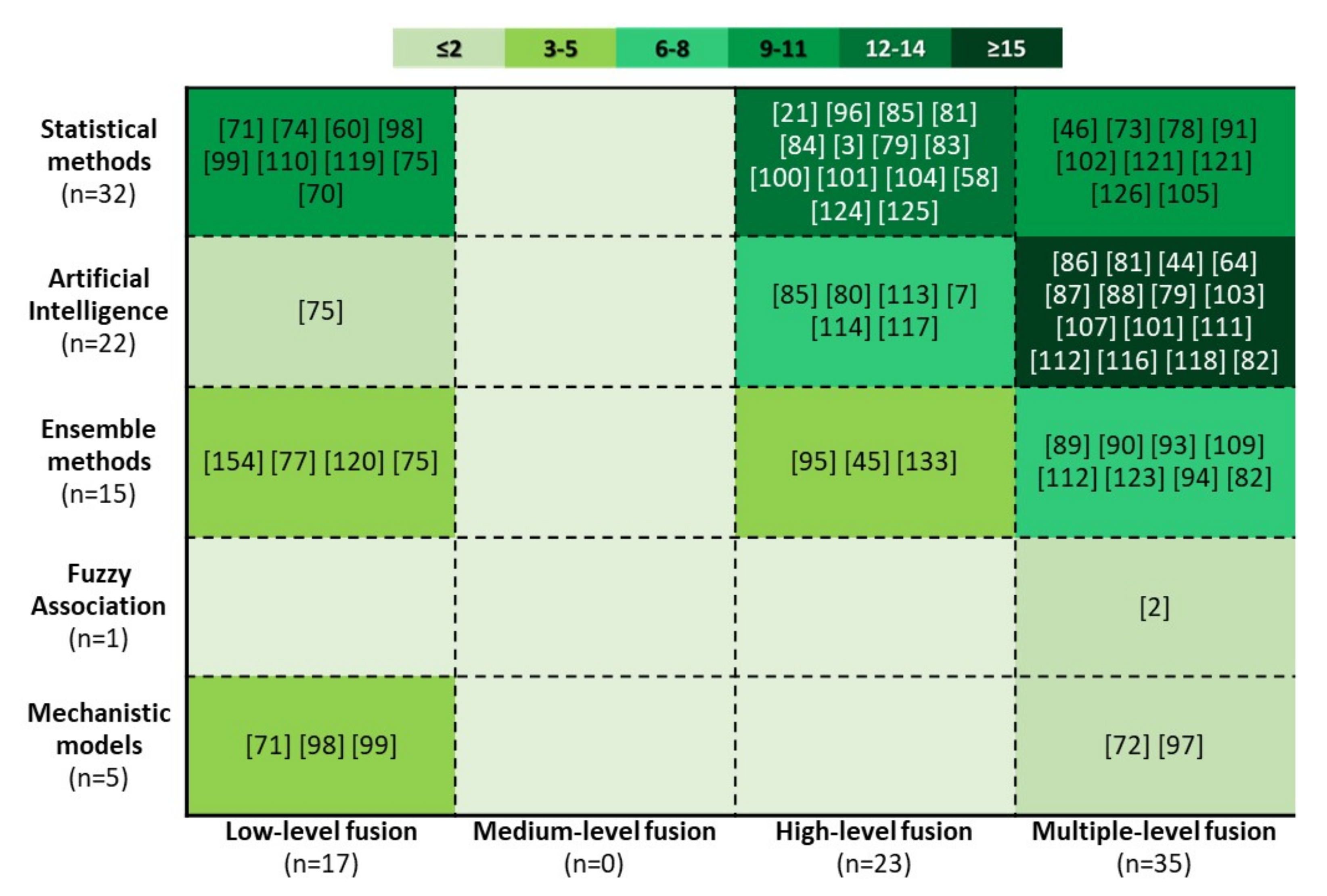
4.5. Data Fusion Models and Evaluation Approaches

A significant range of algorithms was identified Figure 9, attempting to assimilate both sensing types into a classification (n = 43/66) or a regression/correlation schema (n = 17/66) [18]. The majority of the articles avoided using clustering methods, as in most cases (n = 57|86%) crowdsourced data were collected to generate the reference measurements with which the models were trained. Only eight articles [77,80,84,95,110,116,117,154] exploited the data as an additional feature in order to achieve a higher performance rate. Most proposed methods fused data from multiple sensors and in different data formats. The articles using High-level (HF) or Multiple-level fusion (MUF) are the majority (77%), further corresponding to (n = 35) for MUF, (n = 23) for HF and (n = 17) for low data fusion, LF. There were no articles referring to the medium data fusion level (MF). Even in articles dealing with feature extraction (e.g., shapes, textural objects, and others), the crowdsourced data contain labels with certain information, and as such, belong to the MUF or HF categories [114].
According to Figure 9, 32 studies chose to use traditional models, including spatial associations and significant statistical tests [21,46,69,91,92,104,121,125], regression and spatial interpolation models with a single or multiple explanatory variables [60,69,73,74,75,110,119,122,124] probabilistic and decision making models [3,98,99,102]. Classification problems were addressed in object-based [79] and pixel-based schema with the first providing additional image information about the scene, such as shape, length, and spectral details [164]. Empirical rule-based [75,105] and statistical models, such as logistic regression predicted models [57,100,101,126] were explored in four cases [83,84,85,96] using the spatial proximity of model’s predictors. Advance machine- and deep-learning techniques were adopted in 22 articles, incorporating high-level features or features from various data fusion levels (i.e., pixel-decision DF, object-decision DF), while 15 studies introduced ensemble models, allowing multiple classifiers to complement each other and overcome limitations in performance gap and small training instances [89]. Three articles [71,72,97] integrated satellite and crowdsourced data into physical models. Two additional cases [98,99] demonstrated the usefulness of the assimilated EO/CS observations in the flood model predictions, as they give more updated, accurate and less sparse observations. Those articles are listed in both statistical and mechanistic models categories, as the assimilation of EO and CS data produced outputs at two stages, with the first to be the input of the second approach.
In the following sections, an overview of the most noteworthy findings in the data fusion models is given, commenting on their effectiveness and evaluation performance. During this process, comparisons among different evaluation metrics’ rates have been made and documented. Appendix A (Table A1, Table A2, Table A3, Table A4, Table A5, Table A6, Table A7 and Table A8) presents the critical characteristics of each such article, and the evaluation metrics and validation methods used to verify the efficacy of the DF methods.

4.5.1. Low-Level Data Fusion Based on Supervised Learning

Several studies showed a preference to employ linear regression methods [69,110,119] to predict variations in collected values and relations among the explanatory variables and the predicted values, replacing the reference dataset in unknown areas. Furthermore, the type 2 regression (i.e., major axis regression) was found in Elmore et al.’s [74] article, dealing with cases, where both the predicted and explanatory variables are constructed with uncertainty. The change point estimation model was suggested by two articles [60,75] as a method to estimate the changing patterns over time-series of spectrally derived vegetation observations (e.g., MODIS EVI). The idea behind this model is to estimate the changing points in the slope of the fitted line and associate them with the key turning points of vegetation phenological behaviour. Following the same rationale, in the second article, five more empirical rule-based methods were tested, i.e., amplitude threshold, the first, second and third-order derivative, and the relative changing rate, defining the end and start of season phenological dates when the EVI values reached their first local maximum and minimum, respectively. Non-linear associations and complex patterns emphasised the need to utilise advanced machine learning methods (e.g., neural networks—NN [75]) and ensemble models (e.g., random forest regression) [75,154]. Venter et al. [120] supported the use of the RF, as it has been proven more accurate in Tair predictions (RMSE = 8 C and R 2 > 0.5 ) compared to the ordinary least squares (OLS) and support vector machines (SVM). In three articles [77,120,154] an iterative bagging approach was applied in order to decrease the correlation between different tree pairs, avoiding to affect the variance. In Liu’s et al. articles [77,154] validation procedures such as the feature importance testing and the out-of-bag error gave updated predictions achieving a lower estimated error. Continuing, spatial interpolation methods of multivariate linear regression kriging and co-kriging [69] were able to verify the relation of the backscatter signal and the soil moisture, giving better results when predictions are performed in a single land-use type. The leave-one-out cross-validation showcased the significant superiority of the regression kriging with the Root-Mean-Square Error (RMSE) values to reach the accepted scores according to the literature (i.e., >3).
Data assimilation methods with multi-sensory data were explored, giving more accurate data inputs to physical models’ calibrations. Two articles [98,99] applied the sequential DA model of Kalman Filter (KF) to estimate the unknown model’s states-vector based on available observations at each time step. In the above cases, the KF formulated an ensemble model of physical and crowdsourced observations, generating real-time updates according to error’s distribution at each time. Under the same concept, Mehdipoor et al. [71] used the simulated annealing (SA) probabilistic optimisation algorithm to define the optimum set of coefficients for the three SPP models, i.e., the extended spring indices–SI-xLM, the thermal time—TT, and the photothermal time—PTT. 2-sided p-value significant tests and the validation metrics of RMSE and Mean Absolute Error (MAE) illustrated a more efficient performance with the SI-xLM (RMSE = 12 DOY), notifying, on the contrary, the need for spatio-temporal validation processes in order to gain knowledge of variations in different regions. Four rule-based classification algorithms (i.e., RIPPER, PART, M5Rules, and OneR) were applied in [116], following the “divide-and-conquer” training strategy (Table 9). In this article it is reported that the rule-based methods are more suitable in regions with rough topography, as in these cases, models as the KF are unable to perform well.

4.5.2. High-Level Data Fusion Based on Supervised Learning

Uncertainties in spatial and thematic precision and outdated information at coarser resolution are the common factors that drove the research community to investigate the efficiency of hybrid and fused products, (Table 10). Hence, 6 articles [3,21,92,104,124,125] analysed the EO- or CS-driven LC data using statistical and spatial methods, such as spearman rank correlations tests [124], spatial similarity indices [92], spatial labelling aggregations on a predefined area [125] and the majority of voting classifiers [3,21,125]. Furthermore, geostatistical methods such as the hotspot analysis (Getis–Ord statistics and Kernel interpolation with Barriers (KIB)) was applied by Panteras and Cervone [94] to estimate the spatial distribution of flooded regions. Multivariate logistic regression was adopted in three cases [57,100,101], aiming to associate different factors (denoted as pre-disposal factors) with the likelihood of a natural hazard event. Generalized linear models (glm) with the Bernoulli distribution [101] were applied, as well as a data harmonisation process prior to the factors’ inclusion in the model. Supporting this method, statistical significance tests of Wilcoxon–Mann–Whitney test, Pearson’s correlation coefficient (R), and the backward stepwise approach applying the Wald chi-squared ( χ 2 ) test [57,100], were applied to evaluate the significance of examined variables. Continuing, four articles [83,84,85,96] used the geographic-weighted regression (GWR) model to develop a fused global LC map, which proved a valid method [85] performing marginally better (apparent error rate = 0.115, sensitivity = 0.838 and specificity = 0.925), compared to the most known machine-learning classifiers, such as Nearest Neighbour, Naïve Bayes (NB), and the Classification and Regression Trees (CART). Yet, intense computational effort and the multicollinearities between variables highlighted the need to further explore this method.
In another study [79], an object-based classification (OBC) algorithm was used to explore vegetation cover in domestic areas. Reba and Seto [164] as well as Baker et al. [79], claimed that in cases, where a VHR image is used, the OBC method might perform better even compared to machine-learning methods. Fonte et al. [2] introduced the fuzzy logic approach, in which additional weights were assigned to each variable transforming the preliminary equation, according to the reliability of the dependent variable as per the examined factors. Further, two probabilistic models [80,95] are presented to address inconsistencies in the existing LC products. Gengler and Bogaert [80] explored the Bayesian Data Fusion (BDF) algorithm to generate a hybrid crop classification map, built from an interpolated CS crop map and the CCI-LC product. Hughes et al. [95] introduced expert knowledge into a boosting probability graphical model, namely “cluster graph”, as preliminary input to assist the computation of an LC class likelihood on a given region. According to the model’s definition, the following aspects were determined, (a) a tilled-based computational process, dividing the land cover map into sub-regions, (b) the adoption of the Tobler’s law associating similar LC classes to neighbouring locations, (c) the convergence of the system according to the Kullback–Leibler divergence algorithm, and finally, (d) the validation and uncertainty assessment based on Shannon diversity index.
Four articles [85,87,113,117] examined various methods to assess the efficacy of the proposed algorithm compared to state-of-the-art models or to compare their performance. In these studies both shallow- and deep-learning models were used, with the first category to include non-linear and non-parametric ML models of the Support Vector Machine (SVM) based on Radial Basis Function (RBF), RF, and k-Nearest Neighbour (kNN). Examining the performance of these methods, the SVM-RBF had the best classification results (OA = 60.18%). Moving to the deep-learning models, two articles [113,117] used Convolution Neural Networks (CNN) models, as they are able to process multidimensional data and to discriminate complex features and patterns [165]. According to Guo et al. [166] the general pipeline of the CNN consists of three neural layers, (a) the convolution layer that utilises different kernels to convolve the image, (b) the pooling layer to reduce the dimensions of the image, and (c) the fully connected layer, which converts the 2D image-space into a 1D feature vector. In the first article [113], the most known CNN schemes were used, such as the LeNet, the AlexNet, and the VggNet to generate building and road network classification maps. A typical LeNet architecture [167] is defined by two layers using ReLU as the activation function, two fully-connected (FC)-Dropout-ReLU layers, and one softmax or logistic regression classifier. In each convolutional layer, the ReLU function truncates all the negative values to zero and leaves the positive values unchanged, whereas the max-pooling kernel operator is responsible for the dimensional reduction of each image layer, preventing the model from overfitting [115]. Following a similar architecture, the AlexNet [168] and the VggNet [169] incorporate more hidden Conv-ReLU layers [113]. In this experiment, the LeNet-CNN had the highest performance, whereas all of them had issues in the road map extraction, whatever the evaluation metric selected (i.e., F1, Accuracy, and AUC).
Subsequently, a refined version of the U-Net CNN architecture was designed by Li et al. [117], formulating two experiments. The first, referred to as input-based data fusion model, concatenated the extracted CS-road and RS-road features and then trained the images to extract the road network, whereas in the second case, both CS- and RS-road feature datasets are separately trained using the refined U-Net model (RUNET), and then the models’ output was fused according to a certain weight. In the RUNET architecture, two modifications were made; first, excluding the first and the last convolutional stages leading to a reduced complexity, and the second using a rectangle convolution kernel at each stage instead of the square kernel, considered more suitable for the geometrical shapes of the roads. The input-based RUNET model performed better (Sensitivity = 0.840 and OA = 0.672), compared to the state-of-the-art CNN models for road extraction, e.g., LinkNet34, D-LinkNet34 and U-Net, but had challenges in shorter road segments. The last two articles incorporated the transfer learning technology using datasets of the same type [170], to construct larger datasets [171]. Finally, the Single Shot Detection (SDD) network was applied in the Herfort et al.’s [7] study, in order to extract the human settlements with lower effort. The SDD networks follow the tilling concept, where the model is trained in determining boxes. This way, the feature maps are learned to be responsive in particular scales. Additional experiments were performed to identify both the spatial and the non-spatial characteristics of the misclassifications, applying Scott’s rule [172], to calculate the probability of a task to be misclassified. This method was evaluated introducing various metrics, such as false negatives (FN), false positives (FP), true negatives (TN), and true positives (TP), specificity (TNR), sensitivity (TPR), accuracy (ACC), and the Matthews correlation coefficient (MCC). In particular, the MCC was used as an alternative metric of F1 and precision, as the latter have been noted to provide highly biased outcomes for imbalanced datasets [173].

4.5.3. Multiple-Level Data Fusion Based on Supervised Learning

Similar methodologies are proposed in the MUF level, (Table 11), using data with undefined characteristics (e.g., unclassified satellite images) or data formulated at a higher level (i.e., decision level). Such articles exploit numerical models, such as the weather research forecasting model (WRF) [97], three Spring Plant Phenology models (i.e., Spring warming model, Sequential model, and Alternating and parallel model) [72], and the 1D flood simulation model [105], as well as data-driven approaches. Examples of the latter are traditional statistical methods, such as linear regression predictions or correlations [73,78,122], non-parametric significance tests (e.g., pairwise two-sided Wilcoxon-Mann-Whitney test [121]), as well as hybrid classification methods [46,91]. Referring to the latter, preliminary decision maps were obtained using pattern-recognition techniques (i.e., OBIA) [46], clustering models (“Iterative Self-Organizing Data Analysis Techniques A”-ISODATA) [91], which are calibrated based on crowds decisions. In particular, in Vahildi et al.’s [46] study, a citizen science campaign was designed including local groups of civil engineer students, to identify segments in the EO-VHR image, where orchard trees potentially existed. Accordingly, the Template-Matching (TM) algorithm was implemented, assisted by Tobler’s law (indicated the similarity of neighbouring trees), and identified the orchards’ parcels along with their properties (e.g., tree height, growth, etc.). Binary classification models were identified in two articles; the first deploying a logistic regression model [126], and the second the Bayesian probabilistic method, “Weights-of-Evidence”(WoE) [102]. Both cases introduced multiple geospatial variables, obtained from both the CS and RS data and established relations between them and the presence/absence of an incidence. The most widely used probabilistic classification method, that of maximum likelihood, was utilised by Sitthi et al. [88] in order to produce a LC map over Sapporo city, achieving an overall accuracy of 70% and kappa-coefficient of 0.65.
Furthermore, eleven articles [45,81,82,89,90,93,94,109,112,136] opted to use the RF classifier, with all of them focusing their experiments on classification tasks. The RF is an assemblage algorithm that uses a set of decision trees (i.e., CART) to make predictions [174]. Due to its generalised performance, the resistance in noisy datasets, the resilience to overfit [45], the monotonic transformation allowing to avoid the scaling process, and the high prediction accuracy, RF has attracted much attention in the field of remote sensing [175]. In RF, two parameters are taken into account, namely the maximum number of trees that will be generated (Ntree) and the number of the variables that will be selected and tested for the best fit (Mtry). Koskinen et al. [81] used 150 trees to calculate the forest area prediction with an OA equal to 85 ± 2%. Johnson and Iizuka [45] and Fonte et al. [94] set their model with a random selection of variables at each decision node and used 500 trees, thus reducing effects of class imbalance during the training phase. Belgiu and Dragut [112] indicated that the majority of studies use 500 trees, as it ensures that the error is stabilised before the 500th tree. Thornhill et al. [123] applied a random subset of each variable and the mean decrease in accuracy (MDA) to identify the importance among the examined variables. The MDA leverages the internal cross-validation technique of the out-of-bag (OOB) error [176]. Frank et al. [109] validated the performance of the RF algorithm using only certain features, proving that additional features can assist in noise resistance, as the algorithm performed with a lower drop. Wang et al. [94] tried to discriminate the crop types in small-holding parcels in India, leveraging the RF classifier and the seasonal patterns of the Sentinel-1 and 2 data values. Specifically, a discrete Fourier transform, also known as a “harmonic regression”, was applied to S2 observations, even at cloudy images.
Additional DT and ensemble DT learners were found in the examined literature, including the CART [96] and the multivariate C.45 DT classifier (denoted in Weka as J48) [45], the AdaBoost [112], which according to Miao et al. [177] is based on the C5.0 DT algorithm, Rotation Forest (RoF), and Canonical Correlation Forests (CCFs) [89]. RoFs is an ensemble classification method, introduced by Rodriguez et al., showing to outperform the most known ensemble methods (e.g., Bagging, AdaBoost, and RF) [175], with a significant margin. In the CCFs [178], a Canonical Correlation Analysis (CCA) is applied to find the maximum correlations between the features and the class labels. An ensemble-based classifier was developed by Yokoya et al. [89], who combined three state-of-the-art models; CNN (3 layers with ReLU to be the activation function), RF, and gradient boosting machines (GBM) under two frameworks; the first fusing relevant features and the second fusing models’ predictions into a LCZ map. The Markov random field (MRF) was applied as a post-processing spatial smoothing filter, increasing the OA by 7.1% and the kappa-coefficient by 0.08. Additional ML models were identified such as the k-NN [107] and the SVM-RBF [44,81] classification, and the space-partitioning data structure method of the kd-tree-based hierarchical clustering [117]. In the K-NN the Mahalanobis distance was used instead of the Euclidean distance as it provides a better estimation, due to its ability to identify possible correlations and trends among the features. In the presented study, the CCA was applied to investigate the relation among the explanatory variables and the predicted ones.
Several DCNN techniques appeared in eight articles [64,86,94,103,112,114,115] intending to extract image contents related to crop types and urbanised elements, such as urban land use interpretations, archaeological monuments and others. Starting with the first article, a variant of the fully-connected CNN (FCN) was adopted by Kaiser et. al [115], generating a spatially structured labelled image of noisy crowdsourced data. The FCN has the ability to convolve transforming the pixels into 1D label probabilities, and subsequently, deconvolve to gain the initial image size. The model was trained in equally sized mini-batches using the stochastic gradient descent, reaching an average F1-score of 0.84. Lambers et al. [118] identified the Dutch archaeological sites, using an adapted version of the object-detection and image classification CNN denoted as Region-based CNN or Regions with CNN features (R-CNN). In particular, within the R-CNN model, the object identification is conducted at the beginning, generating the required features, which are then fed into the SVM classifier to determine the credibility of the objects. Furthermore, the Dropout strategy was adopted by two articles [112,114] omitting feature detectors that could lead to complex co-adaptations over the training data and model overfitting [166]. In the first study, Chew et al. [112] predicted the probabilities of presence/absence of a residency with the CNN performance exceeding 85%. The transfer learning approach was subsequently used and tested over the pre-trained Inception V3 and VGG16 networks and several shallow-learning models. Zhao et al. [114] designed a 5-layer CNN using a feedforward activation function and the softmax algorithm, predicting labels over unknown semantic EO-elements. Wang et al. [94] constructed two CNN models of 1 and 3 dimensions, exploiting both the spatial and the temporal dimensions over GCVI time-series. Structuring the 1D-CNN architecture, a max-pooling convolutional model at the size of 18 rows (14 S2 features and 4 S1 features) and 365 columns is comprised of multiple convolutional layers and with each layer to use the ReLU. The cross-entropy loss function was used during the training to provide the best-fitted model, and therefore diverse crop types. Attempting to integrate both the spatial and temporal dimensions in the CNN model, a 3D-UNet segmentation network was also tested, exploring the spectral information through time and the corresponding pixels’ behaviour at the maximum distance of 200 m. However, evaluation metrics show that the 1D-CNN slightly produced better results, while a potential reason for this seems to be the higher computational time and the greater number of hyperparameters. Additional variations in CNN algorithms such as the AlexNet, VGGNet, GoogLeNet, ResNet, and the ResNet34 were found in Li et al. [58] and Wiesner-Hanks et al. [86], respectively. Finally, the Generative Adversarial Networks (GAN) model was exploited by Ahmad et al. [103], aiming to detect the flooded regions over crowd selected satellite scenes. According to the aforementioned article, GANs can be considered as unsupervised classification learners, consisting of two competitive NNs. More details on GANs models can be found in Abdollahi et al.’s StoA review [179].

5. Discussion

Within this scoping review, we attempted to provide a holistic overview on research studies assimilating information acquired by Earth Observation and Crowdsourced/Citizen Science data. We have comprehensively reviewed the selected articles according to the collected measurements, the sensors and technological tools or equipment which were used, and the methods that attempted to transform these data into meaningful information regarding the research problems at hand. We adopted a scoping review methodological framework, as a systematic literature review was neither applicable nor realistic, due to the diverse nature of the scope of referenced articles. These variations make the quantitative analysis and comparisons a challenge, illustrating sometimes the loose connections among articles. Concluding, this scoping review aimed to extend previous outcomes [20,52], highlighting gaps and future directions, in research domains that have not been explored so far. Being in line with the previous works, we shall claim that to the best of our knowledge this is the first literature review that examined the data/tools/algorithms and their association withdata fusion types, demonstrating their use and performance in given scenarios. Based on the examined categories, we summarise our review in the following sections.

5.1. General Characteristics of This Scoping Review

This scoping review found that 66 articles (3%, 66/2205) showcased models that integrated observations from EO sensors and citizens and verified their accuracy with specific evaluation metrics. More than half of the studies (e.g., initially 189 articles, from which we only kept 66) were excluded during the full-text screening process, as they did not fulfil the inclusion of both data sources in the models. In most cases, one of the two examined data sources was exploited for the training process, with the second contributing to the evaluation of model’s performance. Observing the number of published articles in the examined years, we have observed an increase in using these data and generating hybrid forms of them. Moreover, both EO and CS data are denoted as “low-cost” solutions, adopted even in countries with limited resources. Indeed, in citizen science projects, the implementation costs are significantly lower, compared to the traditional methods, which are often cumbersome and costly (i.e., costs for the equipment, the development and maintenance of technological solutions, and the data collection campaigns) [180]. However, many studies showed their interdependency with reference data, predominately generated by experts (i.e., researchers, or national administrative datasets, and statistics), indicating that they are not in the position at this stage to replace more mainstream data streams (in situ, authoritative data).

5.2. Datasets’ Uncertainties and Future Trends

5.2.1. Discovering the Advances of Using EO-Satellite Data in Uncommon Applications

The unavailability of open and frequent satellite data is responsible for the high number of studies that opted to overcome this challenge with the integration of crowdsourced data. As Ghermandi and Sinclair [35] stated, at this moment, passive crowdsensing is able to provide great results in (near) real-time, generating new data sources that could complement EO data with close to real time observations. Additional factors such as clouds, outdated scenes, or the complete absence of observations in remote regions have been noted as the most common limitations in Remote Sensing. The Savitzky-Golay filter is also used in time-series models to fill up the cloudy or missing data, applying a 7 point median moving method [75]. Moreover, the so-called “brute force approach” [45] has been proposed, noting that a greater volume of data could overcome noise issues related to clouds, haze, and shadows resulting from the spectral variations in regions with intense inclinations. This approach was applied only with data by the same satellite sensor [90] or explicitly with sensors, which monitor the same spectral range [104].
On the other hand, articles rarely incorporated SAR data in their analysis. Johnson et al. [91] have stated that, in addition to the advantage of SAR sensors to acquire data in every weather condition, they are sensitive to the vegetation structure, as microwaves at specific wavelengths (e.g., L-band) can penetrate the vegetation canopy receiving information of stems and branches. Recent studies have examined the explicit use of the polarimetric [181], as well as the interferometric synthetic aperture radar (InSAR) data to discriminate different backscatter behaviours of vegetation types, such as forests, crop types, etc. [182]. One of the greatest challenges of using SAR data so far was the geometric distortions (e.g., foreshortening, layover, shadowing), caused by the local topography and the right orientation of the satellite. A solution to these variations in the backscatter signal is the terrain-flattened algorithm that can be used to reduce the terrain effects and thus to retrieve “flattened” gamma observations [156]. Complementary studies were even able to tackle the cloud occurrence problem in optical sensors, by fusing SAR and MSI data. Specifically, the DSen2-CR model was based on an image reconstruction task, aiming to predict the missing pixels, denoting as missing the ones covered by clouds. Moreover, we observed that researchers have formulated their models with data from satellite missions that are at the end of their operation. One reason for this is that in some cases it was important to receive knowledge regarding the temporal change of the environment, and thus satellite missions such as the Landsat (revealed in most of the studies) were used the most, as the whole mission (from Landsat 4 to 8) was designed with the same characteristics, enabling time-series observations. However, we claim that the StoA satellite missions, such as the Sentinel missions and the Cube-based platforms (e.g., PlanetScope), give a new challenge in the analysis of this countless data volumes and new perspectives regarding the possibility of observations almost on daily basis.

5.2.2. Addressing the Data Scarcity

Massive volumes of data capture every single spot on earth and this encourages finding new methods of generating annotated data. Nevertheless, the involvement of citizens in this process has been characterised as prone to erroneous judgements, with the citizens revealing additional limitations such as lack of experience, high level of complexity and lack of interest. Subsequently, another restriction in the CS data concerns the preservation of data accessibility. Usually, after the end of the participatory campaign, the acquisition of crowdsourced measurements simply ends, which in some cases (e.g., soil erosion, land cover change, etc.) might not cause a significant consequence, as the monitoring of such kind of phenomena is not necessary to be continuous. Contrarily, in time-series observations or during critical events, such as in air quality, natural hazard rapid events (e.g., floods, earthquakes, fires, etc.) the absence of such information is of paramount importance. On the contrary, referencing other sources of information, such as social media, users effortlessly share important information about the things that matter, usually accompanied by information on time, place, emotions, describing the level of emergency. According to Owuor et al. [183] in 2020 the number of citizens that had access to a personal social media account had reached more than half of the globe’s population. Social media could be characterised as a less labour-intensive, less costly, and less time-consuming approach, and certainly, a scalable approach, as it can be applied at large scales, and at any time and location [35]. In the plethora of applications, social media could assist in the direct provision of critical information, closing the gap of the so far coarse satellite data acquisition. In addition to the general tendency to describe social media as a satisfactory data source, limitations of citizen-generated news, the potential data loss in cases of internet connection absence [104], and the uncertainty of the credibility of such content revealed the need to address the lack of control that still exists [100].
From the model’s perspective, several studies (n = 8|[7,64,112,113,114,115,117,118]) applied the transfer learning method (or domain adaptation [184]), as a potential solution to overcome the sparse and small reference data. The major benefit of this method is that with limited data samples, the model can be trained and fine-tuned, achieving optimal performances in every new task. Yuan et al. [165] mentioned that the transfer learning (TL) framework can be applied using two models; the regional-based TL model, which generates a robust model that can be adapted in various regions, and the data-based TL model that attempts to solve the problem of model generalisation and train with features of multiple sensor images (indicating both satellites and the crowds). However, one limitation was discussed by Chen et al. [113], in cases where the examined objects (e.g., buildings) reveal similar spectral response with neighbouring objects (e.g., the road network) or a completely different because of the diversity of the materials that are used. Both cases are met in low-income regions as a substantial percentage of the urban population living in slums, which are constructed with bricks and other spectrally similar materials to unpaved roads. Additionally, the active learning (AL) algorithm was adopted by two studies [87,113] with the first including both TL and AL in the deep-learning DF model. AL algorithms propose an iterative process of data querying in order to identify the most representative data, using only a small data sample. AL has been applied in studies that lacked labelled data, giving users the samples that had the higher chance of being correctly annotated [87]. On the contrary, two challenges are observed when the AL and DL are incorporated: i.e., the labelling cost, as the AL initiates the training process with a small amount of data, and the data uncertainty, on which the AL model is based. An additional constraint is the data shortage of features. Obtaining training data from existing generalised datasets was adopted in most articles, including data augmentation schemes of image rotations, features with certain properties (e.g., spectral indices, textural features) and the use of generalised datasets (e.g gold-standard benchmark datasets). In addition, deep-learning models, such as the Fast Region-Based CNN or Faster R-CNN [118], the You-Only-Look-Once (YOLO), and the Single-Shot-Detection (SSD) [7], have been introduced to reduce the burden of manual annotation in object detection. Nevertheless, a growing research field targets the development of more elaborate techniques to generate accurate training data that could assist models to perform more efficient predictions.

5.2.3. Data Fusion Leveraging on EO and CS Data

Reviewing the literature, we found that the majority of studies combines EO and CS data with the ultimate aim to develop a model for a specific thematic domain, whereas fewer articles aimed to address “data imperfection” of one of the two data sources. Only Panteras and Cervone [104] exploited the increased temporal resolution of the crowdsourced data, to close the temporal gaps among two consecutive satellite data acquisitions. Section 4.5 verifies this assumption, claiming that in most studies the crowdsourced data were used to generate knowledge in cases, where certain information is not available. In these cases, the crowdsourced information is offered at the highest level of their semantic content, whereas any traditional DF model has difficulties in combining such information with EO-data, as they are described by semantic contents of different levels. Due to this fact, the majority of the articles (n = 35) were assigned to the last level of data fusion.
Considering the DF algorithms, we unexpectedly observed that traditional algorithms still gain significant attention (42.7%), comprising mainly the low- and high-level DF categories. In many articles, models gained knowledge regarding the associations among the two data sources, and preliminary predictions (i.e., linear regression) in unknown areas. Within this category, the GWR had the highest performance in all studies. Additional non-linear extensions of the GWR model, such as the GWR within the artificial neural networks [185] is considered a very promising method. Furthermore, urban applications exhibit a preference in CNN models using satellite imageries at the highest spatial resolution level. Global- or regional-scale applications adopted both data and algorithms with lower computational demands, e.g., geostatistical, and machine-learning models. In general, pre-defined features with coarser characteristics cannot detect objects over a VHR image, when traditional ML algorithms are applied. To remedy this, deep learning strategies can overcome such limitations, enabling to classify popular geospatial datasets [114]. According to Guo et al. [166], deep-learning models have the ability to learn high-level features and be tolerant in heterogeneous and noisy data. Definitely, the existence of the CS and the CNN in the same framework opens a new intriguing possibility to address the enormous demand for annotated training datasets.
Moreover, many models treated data quality as the most important aspect of their research, since various experiments, statistical tests, and evaluation metrics were found across the literature. Experiments were usually conducted to test their theory or to prove the superiority of the model against the StoA algorithms. However, we found two studies [82,113] that integrated two additional metrics for the evaluation of the implemented method, the computational runtime (computed in hours of labelling conduction) and the overall labour (% of the representative images for annotation). The corresponding articles [82,86,113,117] attempted to accelerate the computational process of model training with hardware modules, such as NVIDIA GPUs (i.e., GeForce GTX1080 Ti, TITAN-X, GTX1070 Ti, and Tesla K80) and parallel computing platforms, such as the NVIDIA-docker images [113], and the Hadoop map-reduce framework [111]. Applications that avoided deploying a central workstation explored the computational capabilities of the Google Earth Engine (GEE) cloud-based platform [45,81,82,90]. Within the GEE environment, various combinations of EO datasets at multiple scales and temporal solutions may be accessed, and further generate training datasets for the StoA ML algorithms of CART, RF, NB and SVM. The cloud-based satellite repository of Amazon Web Service (AWS) was used by Yokoya et al. [89] to download the Sentinel-2 archive dataset, which was resampled at 100 m resolution. Li et al. [117] generated and publicly shared a large-scale training dataset, leveraging the GeoServer (http://geoserver.org/; accessed on 28 February 2022) and the use of the Open Geospatial Consortium (OGC) compliant Web Map Service (WMS).
A challenging but rather necessary direction for the data fusion models is to move forward from the evaluation of the model’s accuracy to its adaptation to different regions, and with different datasets. Following this pathway, we identified five articles [64,89,112,113,115] that tested the reproducibility of their approach. In all cases, the models were evaluated with respect to the effect that changes in the training dataset have in the classification task. In this context, a very interesting direction would be to explore synergies among the physical models and the ML/DL. Being aligned with Yuang et al.’s [165] recommendations, this integration could be achieved in the following ways: using the DL to save the enormous computational cost that the physical model simulations require; the calibration of physical model’s outputs with data-driven models to eliminate uncertainties of the input data parameters, and, last, the physics-constrained modelling to achieve an improved optimisation of model’s loss function, and therefore a better understanding of the intermediate processes that occur in the observed phenomenon.

5.2.4. Crowdsourcing Data Curation Challenges and Future Trends

Ensuring the provision of accurate observation from citizens remains a predominant concern of the scientific community, when VGI data are used. However, the precise collection of reference labels of VGI data is still challenging, as it tends to be biased or reveal spatial and thematic discrepancies [186]. In the reviewed articles, class/data imbalance was observed, with the extracted datasets remaining noisy, leading to a lower classification accuracy [113]. Johnson et al. [91] admitted that the inaccurate or limited data provision and the enormous data quantity could also lead to lower performances because both the data and the reference samples must be identically increased. From our perspective, the ability to assess the quality of the CS observations “on-the-spot” during data collection campaigns seems to be an emerging trend. In the 5G era, the increasing need for emergent crowdsourcing applications promotes the use of decentralised mobile systems, as they can consume in real-time the “wisdom of the crowds” and provide a direct validation mechanism [187]. Eventually, immersive platforms (e.g., Virtual Reality (VR)/Augmented Reality (AR)) could have a critical role in citizens’ engagement and training process. AR/VR mobile or web applications could be the “virtual globes” that could assist citizens in familiarising themselves with the crowdsourcing task and thus provide less noisy measurements [188].
As it was observed in the majority of articles, an unorthodox phenomenon is still present; VGI data is on one hand embraced by scientists as the new and auspicious source of information and, on the other hand, is frequently criticised for their discrepancies in quality. Several approaches have been proposed to overcome this challenge, and are described in detail in Section 4.4, including initial statistical methods (e.g., the majority of voting, etc.), probabilities (Naïve Bayes binary classification), and the more complex frameworks of deep-learning NNs. However, a small number of articles investigated the impact of the active involvement of citizens and the behavioural and emotional factors that could contribute to an influential citizens’ engagement. This way, it might be fruitful to shape the direction of future research towards the identification of these societal needs. Ideally, participation in CS projects should have a goal to strengthen citizens’ trust in science and encourage multi-stakeholder partnerships. In this direction, it is mandatory to prioritise citizens’ concerns and apply methods that could obtain a better understanding of the engaged citizens. Such scenarios can result to person-centric approaches (e.g., Latent Class Analysis-LCA and Experience Sampling Method-ESM) [189] and self-assessment questions [136], formulated on the basis of different socioeconomic profiles (i.e., geographic, demographic, non-cognitive and cognitive personal characteristics) [190] and incentives. Therefore, Vohland et al. [189] stated that fruitful outcomes might be generated if such methods could be leveraged in order to trace the heterogeneity in a group or between homogeneous subgroups.
The future of citizen science should go beyond the limits of academic science, in order to be in the position to shape innovation policies and sustainable governmental plans. Social and governmental plans that aim to tangibly contribute to the achievement of Sustainable Development Goals (SDGs) require a collaborative and holistic approach with all the actors (i.e., citizens, policymakers, scientific communities, industrial and social actors) to be engaged. Citizens can offer both bottom-up and top-down perspectives, generating valuable knowledge to scientists and contributing to SDGs’ diversity (bottom-up). On the other hand, citizens may be able to support the initiation of local and global communities that could mobilise governments and businesses to take action (top-down). The role of CS for SDGs has already been acknowledged. Nevertheless, proper transformations of the SDGs to a “common language” is a mandatory activity in order to invest in citizens’ active and continuous involvement [191]. However, without funding schemes and tangible benefits, long-term commitment of CS in SDGs pathways could be at risk. Finally, such activities should be accompanied by relevant dissemination and democratisation of the research findings, targeting the preservation of citizens’ independent views, their social innovation and self-reflection on SDGs [192].

6. Conclusions

In this scoping review, we attempted to provide an overview of the data fusion models that assimilated the remotely sensed and crowdsourced data streams, both of which have emerged as promising, scalable and low-cost ways to provide insights in many domains. The extraordinary increase in articles targeting this research field seized our interest to explore the use cases, where the data is used, the technological equipment and tools, under which a CS survey is leveraged, and eventually, the algorithms that integrate this information, categorised under the data fusion abstraction levels. We carefully reviewed the literature, following the guidelines of the systematic scoping review, and emphasised the strengths and challenges of identified methods overcoming concerns related to data quality, data sparsity, biases related to human cognitive level, and big data related obstacles. Our analysis revealed the necessity of deploying a multi-sensory approach, combining the traditional satellite observations and the next generation StoA missions to confront the spatiotemporal gaps. On the contrary, big data solutions, such as cloud-based platforms, high-performance computing, and datacubes, are a mandatory pathway to take in order to address this countless data volume and the exploitation of EO data in less common research domains.
The beneficial contribution of CS data is depicted across the literature, characterised as a low-cost, low-intensity and scalable data source, which could overcome the limited sample condition. Furthermore, automated object-based or regional-based classifiers and active and transfer learning technologies seemed insightful methods, enabling the provision of an immense amount of annotated training datasets in only a fraction of the time. However, Frank et al. [109] stated their concern regarding the future role of crowdsourcing as the primary receiver of labelling data and the tendency to ultimately substitute users’ in the mapping tasks with automated means [115]. Addressing this conclusion, we attempted to sculpture the future role of citizens by initiating the concepts of collaborative partnerships with multiple actors, person-centered behavioural examination approaches, and most importantly, the democratisation and vulgarisation of scientific-related information, promoting their self-reflection in the existed criticalities and their actual contribution to the mitigation and adaptation policies. Even though the combined exploitation of CS and EO is still underrepresented in the literature, we have shown the huge potential that the aforementioned could achieve. An exciting addition to AI-DF models would be to see the valuable contribution of the geographical information to the quality improvement of the data-driven models and their benefits to the physical environmental models.

Author Contributions

Conceptualization, A.T.; methodology, A.K.; software, A.K.; validation, A.K. and G.T.; formal analysis, A.K.; investigation, A.K. and G.T.; resources, A.A.; writing—original draft preparation, A.K.; writing—review and editing, A.K. and G.T.; visualization, A.K.; supervision, A.T., G.T. and A.A.; project administration, G.T.; funding acquisition, A.A. All authors have read and agreed to the published version of the manuscript.

Funding

This research was funded by the DIONE project under grant number 8703788, supported by European Union’s Horizon 2020 research and innovation program.

Institutional Review Board Statement

Not applicable.

Informed Consent Statement

Not applicable.

Data Availability Statement

Not applicable.

Conflicts of Interest

The authors declare no conflict of interest.

Abbreviations

The following abbreviations are used in this manuscript:
ACCAccuracy
AFOLUAgriculture, Forestry And Other Land Use
AIArtificial Intelligence
ALActive Learning
AlexNetConvolutional Neural Network (CNN) Architecture, designed By Alex Krizhevsky
ALIAdvanced Land Imager
ALSAirborne Laser Scanning
AODAerosol Optical Depth
AOTAerosol Optical Thickness
APIApplication Programming Interface
APSActive Participatory Sensing
ARAugmented Reality
AR66th Assessment Report
ARCAmerican Red Cross
ARDAnalysis-Ready Data
AWSAmazon Web Service
BDFBayesian Data Fusion
BMEBayesian Maximum Entropy
BSIBare Soil Index
BuEIBuilt-Up Index
C/N 0 Carrier-To-Noise Ratio
CARTClassification And Regression Trees
CCClimate Change
CCACanonical Correlation Analysis
CCFCanonical Correlation Forests
CCI-LCClimate Change Initiative Land Cover
CDOMColoured Dissolved Organic Matter
CEOSCommittee On Earth Observation Satellites
CGDCrowdsourced Geographic Data
CGICrowdsourced Geographic Information
chl-aChlorophyll-A
CHMCanopy Height Model
CILCitizen Involved Level
CNNConvolutional Neural Network
COCitizen’s Observatory
CSCitizen Science
CTClassification Task
CTICompound Topographic Index
DAData Assimilation
DBDatabase
DBSCANDensity-Based Spatial Clustering Of Applications With Noise
DCTDigitisation-Conflation Tasks
DEMDigital Elevation Model
DFData Fusion
DMS-OLSDefense Meteorological Satellite Program’s Operational Linescan System
DPDeveloped Platforms
DSMDigital Surface Model
DTMDigital Terrain Model
EOEarth Observation
EO4SDEarth Observation For Sustainable Development
EOSEnd Of Season
EVIEnhanced Vegetation Index
EXIFExchangeable Image File
FAOFood And Agriculture Organization
FCMFuzzy C-Means
FCNFully Connected Neural Network
FETAFast And Effective Aggregator
FNFalse Negative
FPFalse Positive
FUIForel-Ule Colour Index
FWWFreshwater Watch
GANGenerative Adversarial Networks
GBMGradient Boosting Machines
GCCGreen Chromatic Coordinate
GCOSGlobal Climate Observing System
GEEGoogle Earth Engine
GEOGroup On Earth Observations
GEOBIAGeographic Object-Based Image Analysis
GF-2Gaofen-2
GHGGreenhouse Gas
GLC2000Global Land Cover Project
GLCMGrey-Level Co-Occurrence Matrix
glmGeneralized Linear Models
GNSSGlobal Navigation Positioning Systems
GPSGlobal Positioning Systems
GSVGrowing Stock Volume
GUFGlobal Urban Footprint
GUIGraphical User Interface
GWRGeographic-Weighted Regression
HFHigh Data Fusion Level
HITHuman Intelligence Tasks
HOTOSM Team For Humanitarian Mapping Activities
HRSLHigh-Resolution Settlement Layer
HVHorizontal—Vertical Polarisation
IBIIndex-Based Built-Up Index
IIASAInternational Institute For Applied Systems Analysis
Inc/ExcInclusion/Exclusion
InSARInterferometric Synthetic Aperture Radar
IPCCIntergovernmental Panel on Climate Change
ISODATAIterative Self-Organizing Data Analysis Techniques
ISPRSInternational Society for Photogrammetry And Remote Sensing
KDFKernel Density Function
KFKalman Filter
KIBKernel Interpolation with Barriers
kNNK-Nearest Neighbour
LCLand Cover
LCZLocal Climate Zones
LDALatent Dirichlet Allocation
LeNetConvolutional Neural Network (CNN) Structure Proposed By Yann Lecun
LFLow Data Fusion Level
LSTLand Surface Temperature
MADMedian Absolute Deviation
MAEMean Absolute Error
MaxEntMaximum Entropy
MCCMatthews Correlation Coefficient
MCSMobile Crowd-Sensing
MDAMean Decrease in Accuracy
MFMedium Data Fusion Level
MLMachine Learning
MMSMin–Max Scaler
MMUMinimum Mapping Unit
MNDWIModified Normalised Difference Water Index
MNFMinimum Noise Fraction
MODISModerate Resolution Imaging Spectrometer
MRFMarkov Random Field
MTurkAmazon Mechanical Turk
MUFMultiple Data Fusion Level
NBNaïve Bayes
NBARNadir Bidirectional Reflectance Distribution Function-Adjusted Reflectance
NDBINormalised Difference Build-Up Index
NDVINormalised Difference Vegetation Index
NDWINormalised Difference Water Index
NIRNear Infrared
NLPNatural Language Processing
NNNeural Networks
NPNNational Phenology Network
OBCObject-Based Classification
OBIAObject-Based Image Analysis
ODbLOpen Database
OGCOpen Geospatial Consortium
OLSOrdinary Least Squares
OneROne Attribute Rule
OOBOut-Of-Bag
OSMOpenstreetmap
OsmAndOpenstreetmap and the Offline Mobile Maps and Navigation
OSSEObserving System Simulation Experiment
PARTProjective Adaptive Resonance Theory
PCAPrincipal Component Analysis
PCSPassive Crowdsourcing
PEATProgressive Environmental and Agricultural Technologies
PHPhotograph Sharing Services
P M 10 Particulate Matter with Diameters of 10 μ m
P M 2.5 Particulate Matter with Diameters of 2.5 μ m
PRISMParameter-Elevation Regressions on Independent Slopes Model
PTTPhotothermal Time
PWSNPersonal Weather Station Network
QGISQuantum GIS
RBFRadial Basis Function
R-CNNRegions with CNN Features or Region-Based CNN
ReLURectified Linear Unit
ResNetResidual Neural Network
RFRandom Forest
RGBRed-Green-Blue
RIPPERRepeated Incremental Pruning to Produce Error Reduction
RMSERoot Mean Square Error
RoFRotation Forest
RSRemote Sensing
S1Sentinel-1
S2Sentinel-2
SASimulated Annealing
SARSynthetic Aperture Radar
SDSecure Digital
SDDSingle Shot Detection
SFDRRSendai Framework for Disaster Risk Reduction
SHBSecondary Human Behaviour
SI-xLMExtended Spring Indices
SMSocial Media-Networking Services
SMOTESynthetic Minority Oversampling Technique
SoEISoil Index
SOSStart Of Season
SPSmartphones
SPMSuspended Particulate Material
SPoCSum-Pooled Convolutional
SPPSpring Plant Phenology
SSDSingle-Shot-Detection
SSLSignal Strength Loss
SSLRScoping Systematic Literature Review
StoAState-of-the-Art
SVFSky View Factor
SVMSupport Vector Machine
TAITrue-Colour Aerial Imagery
TFLTobler’s First Law Of Geography
TLTransfer Learning
TMTemplate-Matching
TNTrue Negative
TNRSpecificity
TPTrue Positive
TPRSensitivity
TTThermal Time
TWITopographic Wetness Index
UAVUnmanned Aerial Vehicle
UHIUrban Heat Island
UN-SDGUnited Nation-Sustainable Development Goals
USFSUnited States Forest Service
VGGVisual Geometry Group
VGIVolunteer Geographic Information
VHRVery High Resolution
VOCVisual Object Classes
VRVirtual Reality
WHOWorld Health Organisation
WMSWeb Map Service
WNSWireless Network Stations
WoEWeights-of-Evidence
WRFWeather Research Forecasting Model
WSIWeSenseIt
WUDAPTWorld Urban Database and Access Portal Tools
WUIWildland-Urban Interface
YOLOYou-Only-Look-Once

Appendix A

Table A1. Summary table of Vegetation Monitoring studies included in this scoping review. Abstraction levels of data fusion and Technological equipment of CS data collection are described as assisted by the categories and abbreviations presented in Section 3.5.1 and Section 3.5, respectively. Methods are categorised as the following, AI: Artificial Intelligence, S: Statistical method, ES: Ensemble methods, FS: Fuzzy Association, and M: Mechanistic models.
ReferenceEO DataSource of CSDF LevelMethodValidationEvaluation Metric and Score
[79]AerialDP/My Back Yard toolHFGeoBIA/SA manually digitised reference layer and a stratified separation of the dataset was usedOverall Accuracy using Multinomial Law equation (73.5% classification result, and 76.63% CS valid decision)
[154]Satellite/GNSSSensors/GPS receiversLFRF Regression/ESOut-of-Bag error estimation leveraging on reference data of forest attributesRMSEs: mean tree height = 14.77–20.98% Mean DBH = 15.76–22.49%; plot-based basal areas = 15.76% and 33.95%, stem volume and AGB = 27.76–40.55% and 26.21–37.92%; R = 0.7 and 0.8
[77]Satellite/GNSSSensors/GPS receiversLFRF Regression/ESOut-of-Bag error estimation comprising of reference data with forest attributesThe combination of the GLONASS and GPS GNSS signals slightly better results than the single GPS values.
[60]Satellite/MSIDP/NPNLFLinear change point estimation/SGround-based phenological datesRMSE, bias, MAE and Pearson’s R evaluation metrics were used, revealing a weak significance when the CS data were used (Best result: r = 0.24, MAE = 23.0, bias = −14.8, and RMSE = 28.0)
[73]Satellite/MSIDP/PlantWatchMUFL-Regression/SStratification based on the GLC2000 land cover mapGreen-up date RMSE unsystematic (RMSEu) and systematic (RMSEs) were 13.6 to 15.6 days, R and p < 0.0001
[85]Satellite/LULCDP/Geo-WikiHFk-NN, Naïve Bayes, logistic regression, GWR, CART/AI + S10-fold cross validationBinary classification: Apparent error rate (GWR: AER = 0.15), Sensitivity (CART: Sen = 0.844), Specificity (GWR: Spe = 0.925), pairwise McNemar’s statistically significance test (GWR: p = 0.001); % Forest cover: GWR: AER = 0.099, CART: Sen = 0.844, GWR: Spe = 0.927, GWR: p = 0.001
[84]Satellite/LULCDP/Geo-WikiHFGWR/SEqual-area stratified random samplingLULC OA forest recognition (89 %), specificity = 0.93, Sensitivity = 96%; Estimation of % forest cover R 2 = 0.81, RMSE = 19
[83]Satellite/LULCDP/Geo-WikiHFGWR/SValidated with a random distribution of reference dataApparent error % Hybrid predicted dataset = 4 (Best score for Russia), and 5 for the Sakha Republic
[71]Hybrid/in situ and DEMDP/NPNLFSprint Plant Phenolog/MResubstitution error rate between the observed and the estimated daysRMSE and MAE of the Day of the Year (DOY) resulted in 11.48 and 6.61, respectively (Best model)
[3]Satellite/LULCDP/53,000 CS data samples were gathered on the Geo-wiki platformHFConvergence of evidence approach (IDW interpolation)/S(1) Stratified dataset from 2 CS campaigns. Finalised with experts’ evaluation. (2) 1033 pixels with high disagreement randomly classified by 2 experts.(1) Stratified dataset from 2 CS campaigns. Finalised with experts’ evaluation. (2) 1033 pixels with high disagreement randomly classified by 2 experts.
[78]Hybrid/Rainfall Satellite/MSIDP/CS campaign archived in NPNMUFL-Regression Spearman’s correlation, Binary-thresholding classification/S(1) Reference data collected on the field, (2) CLaRe metrics(1) R 2  > 0.5 between field observations and independent variables; (2) T-tests between CLaRe, native and invasive Buffelgrass depicted significant differences. (3) OA Buffelgrass classification was equal to 66–77%, with trade-offs in UA, PA accuracies
[46]Satellite/MSIOther/CS campaignMUFTemplate match binary thresholding/SValidated with reference training samples applying hold-out dividing the dataset in train-testingCompleteness (C = 69.2 to 96.7), Thematic accuracy metrics: positive predictive value (PPV = 0.926 to 1.000), false positive (FDR = 0.037 to 0.550), false negative rate (FNR = 0.033 to 0.308), F1 = 0.545 to 0.964, Positional accuracy metrics: Diameter error for a correctly identified ITC (ed) RMSE for tree crown diameter measurement for crowdsourced observation (RMSEcd = 0.67 to 0.93) and tree crown centroid position measurement (RMSEcc = 0.28 to 1.01)
[86]Aerial/MSIDP/Amazon’s Mechanical TurkMUFResNet34 CNN model/AIHold-out dataset separation in train, validation and test based on [193] methodOA = 0.9741, precision = 0.9351, recall = 0.9694, F1 = 0.9520
[72]Hybrid/MSI and rainfall (gridded and in situ)DPtextbackslash NPN and PH/PhenoCamMUF13 SPPs + Monte Carlo optimisation/Min situ phenological dataBest optimised parameters were determined with 95% confidence intervals for each parameter, using the chi-squared test. AICc was used to select the best model for all the species. R = 0.7–0.8, RMSE = 5–15, and Bias = ±10 days
[81]Satellite/SAR, MSI, DEMOther/2 week CS campaignMUFCART/AIReference data set of 7500 sample points was generated and stratified based on the first stage land cover classesForest plantation area was estimated with high overall accuracy (85%)
[74]Satellite/MSIDP/NPNLFType 2 Regression/S-Non-significant results, R 2 = 0.014; p = 0.052; Rule #1 R 2 = 0.19; p < 0.001 & Rule #2 R 2 = 0.29; p < 0.001. Median MODIS values improved R 2 = 0.67; p < 0.001. Lilac revealed the greatest results R 2 = 0.32–0.73; p < 0.001. R 2 = 0.23 to 0.89 across species.
[80]Satellite/LC productDP/Geo-WikiHFBayesian data fusion (BDF)/AIStratification keeping only those where CS data were at hand (i.e., 500)BDF has proven a suitable method as the log-likelihood ratio ( G 2 ) and the chi-squared ( χ 2 ) were 0.2511 and 5.991, corresponding to a p-value = 0.8820. The OA of the cropland = 98.00%.
[75]Satellite/MSIDP/NPNLF6 S models 1, NN AI and RF regression ES10-fold cross validation with the analogy of 80/20RF outperformed with r = 0.69, WIA = 0.79, MAE = 12.46 days and RMSE = 17.26 days (for deciduous forest)
[82]Satellite/MSI and SARSP/PlantixMUF1D and 3D CNN/AI and RF harmonic coefficients/ESFeature Importance via Permutation; using also governance district statistics(A) 3-crop type classes: Accuracy: 74.2 ± 1.4%, Precision = 75.9 ± 1.7%, Recall = 74.2 ± 1.4%, F1 = 73.7 ± 1.4%; (B) crop-type map accuracy = 72%
1 S: Threshold, amplitude threshold, delayed-moving window, first and higher-order derivate, function fitting method.
Table A2. Summary table of Land Use/Land Cover studies included in this scoping review. Abstraction levels of data fusion and Technological equipment of CS data collection are described as assisted by the categories and abbreviations presented in Section 3.5.1 and Section 3.5, respectively. Methods are categorised as the following, AI: Artificial Intelligence, S: Statistical method, ES: Ensemble methods, FS: Fuzzy Association, and M: Mechanistic models.
ReferenceEO DataSource of CSDF LevelMethodValidationEvaluation Metric and Score
[90]Satellite/MSIDP/OSMMUFCART, RF/AI + ESStratified random validation using ground truth (1), Landsat-based LC maps (2)OA and kappa coefficient of urban land can reach 88.80% and kappa-coefficient 0.74 (1), and 97.08% and 0.92 (2)
[44]Satellite/MSIMUFSVM RBF/AI5-fold CV, using a manually digitized LCOA = 93.4 and kappa coefficient = 0.913
[95]Satellite/LCDP/OSMHFProbabilistic Cluster Graphs/ESResubstitution using the ATKIS national Digital Landscape Model (1:250,000)Scenario 4 with the general class-weighting factor predicted with OA = 78% and kappa: 0.67. Class-wise balanced accuracy produced more accurate results
[96]Satellite/LCDP/Geo-WikiHFLogistic-GWR/SStratification scheme based on Zhao et al. [194] using an independent validation dataset, and 2 Geo-Wiki campaignsGenerated two-hybrid maps with the first to perform better (OA: 87.9 %). The tree-cover land class presented the best results among all classes, in both maps, PA_1: 0.95, UA_1: 0.94 and PA_2: 0.97, UA_2: 0.93
[91]Satellite/SAR and MSIDP/OSMMUFISODATA and Estimation fractional cover of LC/SStratification random sampling approach (50 validation points per LCC class)The confusion matrix of the LCC classification map shows an OA = 90.2%. “Tree cover” and “cropland/grassland” reveal the greatest confusion in change classes.
[88]Satellite/MSIPH/FlickrMUFNaïve Bayes CS LULC, Maximum likelihood/AIStratified the train/testing dataset having an analogy of 70/30LULC (Landsat-5 TM + CS LULC map), with OA and kappa equal to 70% and 0.625, respectively. The accuracy level was mostly driven by urban areas.
[45]Satellite/MSIDP/OSMHFNB, DT-C.45/AI, RF/ES(a) Random Subsampling-Hold out: 50/50 (b) SMOTE stratification methodDT C.45 gave the lowest OA values. In the LULC system, NB achieved OA = 72.0%, followed by RF in the 5 and 4-classes LULC system (OA = 81.0% and OA = 84.0%)
[92]Satellite/MSISM/SINA WEIBO and Baidu DP/OSMHLBinary Thresholding, Similarity Index/SRandom Subsampling-Hold out, based on 289 visual inspected testing parcelsLU Level I classes: OA = 81.04% and kappa-coefficient = 0.78; LU Level II classes: OA = 69.89% and kappa-coefficient = 0.68%
[21]Satellite/MSIOther/Focus groupsHFStatistical analysis/SResubstitution method using reference dataConfusion matrices were computed in the sense of measuring the deviation in LU-class coverage
[89]Satellite/MSIDP/OSMMUFRF (RoFs and DT), XG- Boost, and CNN/ES15 randomly defined training datasets (10 uniformly divided, 5 last extracting 500 samples for all the classesLCZ OA = 74.94%, kappa = 0.71 (the greater score using RF method, and experts handcrafted features). The classification accuracy increased with the imbalanced dataset
[93]Hybrid/MSI and DEMDP/OSMHFRF Classifier/ESRandom Subsampling-Hold out randomly selecting validation points, splitted in training and testing datasetOut-of-bag error = 4.8% and OA = 95.2%, with 95.1% of the forested areas to be correctly classified. Low user’s accuracy of 57.4% was revealed on commercial lands
[136]Satellite/MSIDP/Google EarthMUFRF Classifier/ESReference dataset by LCZ expertOA = 0 to 0.75 (produced by several iterations)
[64]Satellite/MSIDP/OSM SM/FB and TwitterMUFSVM and DCNN/AITransfer performance learning with UC-Merced dataset and 10-fold Cross-ValidationOA is based on the mean and standard deviation of all the results. OA_train = >90% and OA_test = 86.32% and 74.13%
[87]Satellite/MSIDP/Crowd4RSMUFAc-L-PBAL and SVM RBF, RF, k-NN/AI260 labelled samples were provided by RS expertsThree-cross-validation technique of the 3 algorithms. OA = 60.18%, 59.23% and 55%
[2]Satellite/MSIDP/OSMHFFuzzy logic/FSStratified random sampling of 200 points per class5 tests were evaluated with the final one to reveal OA = 70%. Population true proportions (pi) [195], UA and PA per class also calculated.
[94]Satellite/MSIDP/OSMMUFRF Classifier/ESStratified random samplingOA = 78% (study area A) and OA = 69% (study area B)
Table A3. Summary table of Natural Hazards studies included in this scoping review. Abstraction levels of data fusion and Technological equipment of CS data collection are described as assisted by the categories and abbreviations presented in Section 3.5.1 and Section 3.5, respectively. Methods are categorised as the following, AI: Artificial Intelligence, S: Statistical method, ES: Ensemble methods, FS: Fuzzy Association, and M: Mechanistic models.
ReferenceEO DataSource of CSDF LevelMethodValidationEvaluation Metric and Score
[101]Hybrid/Satellite and in situDP/VGI mappers using Google EarthHFMultivariate Logistic regression/SResubstitution DFO mapLog-Likelihood, chi-squared, and p-value tests, revealed −15,952 465.94, and 2.2   ×   10 16 16 for the outside of the city model, and −7534, 273.41 and 2.2   ×   10 16 for the inside.
[110]AerialSensorsLFUnivariate L-Regression/SResubstitution between CS and DOE R 2 = 0.87
[109]AerialDP/QGIS, Web-based eCognitionMUFRF Classifier/ESHold out human-labelled training dataEstimation of feature importance of the model. Pixel-based classification seemed more noise resistant with the AUC to drop 2.02, 7.3, and 0.85% for NAR, label noise and random noise when 40% of the damage is contaminated.
[104]Satellite/DEMSM/TwitterHFGetis–Ord Gi*-statistic/SUsing an elevation thresholdEvaluation of statistical significance based on z-score values ± 1.64
[100]Hybrid/in situ, DEMSM/BaiduHFMultivariate logistic regression/SResubstitution with Wuhan water authority flood risk mapsBackward stepwise significance method (Wald chi-square test = 0.001), AUC = 0.954, asymptotic significance = 0.000
[98]Satellite/DTM, LiDARSM/YouTube and TwitterLFEnKF/SResubstitution using the observed water depth valuesNash–Sutcliffe efficiency (NSE) > 0.90 and R > 0.97 (Best results)
[102]Satellite/MSI, DEMPH/FlickrMUFWoE/SRandom Subsampling-Hold out with 120 pointsROC for Flickr images was 0.6 (train) and 0.55 (test). EO was 0.88 and 0.90, and AUROC posterior = 0.95 and 0.93. Pair-wise conditional independence ratio = 6.38
[103]Satellite/MSIDP/JORD app, SM/Twitter, YouTube, PH/Flickr, GoogleMUFV-GAN/AITwo-fold cross-validation strategyMatthews correlation coefficient for the binary classification = 0.805. OA = 0.913, precision = 0.883, recall = 0.862, specificity = 0.943, and F1 = 0.870
[99]in situSensor, SmartphoneLFKalman Filter/SResubstitution error rate between the reference and simulated values4 experiments were evaluated using NSE and Bias’s indexes. However, no general conclusions can be derived.
[107]Satellite/MSI, DEMSmartphoneMUFMahalanobis K-NN/AILOOCV leveraging on the reference datasetCanonical correlation (F = 2.77 and p < 0.001)), Wilk’s lambda = 0.007. RMSD investigated professional (P), non-professional (NP), raw data (R) and corrected by experts (C) 2
[105]Hybrid/Satellite and in situSmartphoneMUFFlood-fill simulation/Sin situ reference measurements and experts’ quality controlKappa-coefficient = 0 to 0.746
2 Best results: RMSD was estimated for the indicators related to the wildland-urban interface (WUI) fuel model, which are Conifer crown closure (All = 22.5%), Conifer crown base (P = 1.9 m), Suppressed conifers (All = 114.0 stems/ha), Surface vegetation (All = 21.6%), Large woody debris (All = 28.3%), Fine woody debris (All = 33.2%).
Table A4. Summary table of Urban Monitoring studies included in this scoping review. Abstraction levels of data fusion and Technological equipment of CS data collection are described as assisted by the categories and abbreviations presented in Section 3.5.1 and Section 3.5, respectively. Methods are categorised as the following, AI: Artificial Intelligence, S: Statistical method, ES: Ensemble methods, FS: Fuzzy Association, and M: Mechanistic models.
ReferenceEO DataSource of CSDF LevelMethodValidationEvaluation Metric and Score
[57]Satellite/MSIDP/OSMHFLogistic regression/SValidation by expertsOA = 89%, Sensitivity = 73%, Precision = 89%, F1-score = 0.80, and 25% volunteers contribute 80% of the classification result
[115]Satellite/MSIDP/OSMMUFFCN (VGG-16)/AIHold-out equally divided the dataset into train-test-validationThe best model “ISRPS Gold standard data” with average F1 = 0.874, Precision = 0.910, Recall = 0.841 and F1 = 0.913, 0.764, 0.923 for the building, road, and background classes.
[116]Hybrid/GNSS, DEM, LC, AerialSmartphoneLFRIPPER, PART, M5Rule, OneR/AI10-fold Cross-Validation (CV) and Visual inspectionEvaluation of CS traces using Shapiro-Wilk, skewness and kurtosis tests. RIPPER’s best results: Precision = 0.79, recall = 0.79, F1 = 0.79
[113]Satellite/MSIDP/OSM, MapSwipe, OsmAndHLLeNet, AlexNet, VggNet/AIRandom Subsampling Hold-out with MapSwipe and OsmAnd as ground-truthPrecision, Recall, F1, and AUC of combined CS data were higher with an average of 9.0%, 4.0%, and 5.7%
[114]Satellite/MSIDP/OSM; SM/BaiduMUFFCNN, LSTM, RNN (1)/AI; SVM, LDA (2)/AIRandom Subsampling Hold-out (4:1 train/test)OA was increased from 74.13% to 91.44%. Building and road categories were increased by around 1% (1); OA_SVM = 72.5%, LDA = 81.6%, PM = 93.1% (2)
[117]Satellite/MSISmartphone/GNSSHFU-Net, LinkNet, D-LinkNet/AIFusion RS with the outputs of road centerline extractionCompleteness (COM), Correctness (COR) and Quality (Q) equal to 0.761, 0.840, 0.672
[118]Satellite/LiDAROther/Focus Groups and DP/ZooniverseMUFFaster R-CNN/AIModel division in Train, Test, ValidationRecall, Precision, F1, MaF1 evaluation metrics presented in [196]
[111]Satellite/MSIDP/TomnodMUFkd-tree-based hierarchical classification/AIStratification based on population density classes, and reference data, created by citizens’ visual inspectionLogistic and beta regressions were applied for the precision (0.70 ± 0.11) and recall (0.84 ± 0.12) metrics, evaluating the village boundaries of (1) the examined areas, and (2) six cities of the globe. Evaluation of the Population density by the normalised correlation (NC), and the normalised absolute difference (ND).
[7]Satellite/MSIDP/OSM, MapSwipeHFDeepVGI model (Single Shot Detection (SSD) CNN)/AIHold out dataset division in train and test. Maximum training epochs was set to 60,000Specificity, Sensitivity, OA (ACC), Matthew’s correlation coefficient (MCC) metrics. DeepVGI model revealed similar results to MapSwipe, i.e., OA = 91–96%, MCC = 74–84%, specificity = 95–97%, and sensitivity = 81–89%
[112]Hybrid/MSI and LULCDP/OSMMUFBagging CNN, V3, VGG16/ES(1); SL models 3/AI(2)Hold-out (85//15 train/test) using a reference dataset.Ensemble model revealed the best results in both Nigeria and Guatemala, OA_N = 94.4%, OA_G = 96.4%, and F1_N = 92.2%, F1_G = 96.3%. Transfer Learning models performed with OA_N = 93% and OA_G = 95%, Human benchmark (OA_N = 94.5%, OA_G = 96.4%). AdaBoost and logistic regression performed better.
3 7 classification algorithms: Decision trees, Gradient boosting trees, AdaBoost, Random Forest, logistic regression, support vector machines, and k-nearest neighbour.
Table A5. Summary table of Air monitoring studies included in this scoping review. Abstraction levels of data fusion and Technological equipment of CS data collection are described as assisted by the categories and abbreviations presented in Section 3.5.1 and Section 3.5, respectively. Methods are categorised as the following, AI: Artificial Intelligence, S: Statistical method, ES: Ensemble methods, FS: Fuzzy Association, and M: Mechanistic models.
ReferenceEO DataSource of CSDF LevelMethodValidationEvaluation Metric and Score
[121]Hybrid/DEM, LULC and in situSensorsMUFNon-parametric significant tests LCZ/SReference weather stations1-way ANOVA (Kruskal-Wallis test), pairwise 2-sided Wilcoxon-Mann-Whitney and Holm-Bonferroni. Difference CS = 1.0 K and Reference = 1.8 K; Difference between the 2 datasets ± 0.2–2.9 K
[119]Hybrid/in situ and SatelliteSensorsLFL-Regression/Sin situ P M 2.5 US EPA Air Quality concentrations, and Aeronet AOD R 2 = 0.04
[120]Satellite/MSI + LiDARSensorsLFRF Regression; ANOVA test for the explanatory variables/ESHold-out (70/30) with bootstrapping repeatedly occurred 25 timesAnnual mean, daily maximum and minimum Tair can be mapped with an RMSE = 0.52   C, R 2 = 0.5 ), 1.85   C ( R 2 = 0.5 ) and 1.46   C ( R 2 = 0.33 ); Transferability revealed an RMSE = 0.02   C difference.
[97]Hybrid/LULC and in situS/Personal Weather StationMUFWRF model/MCompared with measurements from in situ weather stationsRMSE = 0.04 K and Mean Bias = 0.06 K (p = 0.001). Weak positive correlation (r = 0.28) of the elevation with variations in model’s performance
Table A6. Summary table of Ocean/marine monitoring studies included in this scoping review. Abstraction levels of data fusion and Technological equipment of CS data collection are described as assisted by the categories and abbreviations presented in Section 3.5.1 and Section 3.5, respectively. Methods are categorised as the following, AI: Artificial Intelligence, S: Statistical method, ES: Ensemble methods, FS: Fuzzy Association, and M: Mechanistic models.
ReferenceEO DataSource of CSDF LevelMethodValidationEvaluation Metric and Score
[124]Satellite/MSISmartphoneHFMulti-Linear Regression/S-Spearman rank coefficient; R 2 = 0.25 , 0.32; mean absolute difference = 21 ± 16%, 22 ± 16%), mean difference = 6 ± 26%, 6 ± 27%
[122]Satellite/MSISmartphoneMUFBackward step Multi-Linear-Regression/SField measurementsSpearman rank coefficient; Adjusted R 2 = 0.50 , standard error 0.274 with stream distance weighted mixed forest and urban, and riparian percentage
[123]Satellite/MSI, DEMSensorMUFRF Regression/ESout-of-bag using 10–fold cross-validationTurbidity: OA = 65.8%, kappa = 0.32, Error good—bad evaluation 34.6% and 36.0%; Nitrate: 70.3%, 0.26, 58.8%, 14.7%; Phosphate: 71.8%, 0.39, 50.0%, 22.6%
Table A7. Summary table of Humanitarian and crisis response studies included in this scoping review. Abstraction levels of data fusion and Technological equipment of CS data collection are described as assisted by the categories and abbreviations presented in Section 3.5.1 and Section 3.5, respectively. Methods are categorised as the following, AI: Artificial Intelligence, S: Statistical method, ES: Ensemble methods, FS: Fuzzy Association, and M: Mechanistic models.
ReferenceEO DataSource of CSDF LevelMethodValidationEvaluation Metric and Score
[125]Satellite/MSIDP/ZooniverseHFAveraged density of kilns/SRandom sample selection; Visual inspection by an Independent adjudicatorOA = 99.6%; Error of experts = 0.4%; of CS = 6.1%
[126]Satellite/NightlightsDP/Syria trackerMUFLogistic regression/S-Statistical significance of all models is below 5%. Best model result AIC = 127,967
Table A8. Summary table of Soil moisture studies included in this scoping review. Abstraction levels of data fusion and Technological equipment of CS data collection are described as assisted by the categories and abbreviations presented in Section 3.5.1 and Section 3.5, respectively. Methods are categorised as the following, AI: Artificial Intelligence, S: Statistical method, ES: Ensemble methods, FS: Fuzzy Association, and M: Mechanistic models.
ReferenceEO DataSource of CSDF LevelMethodValidationEvaluation Metric and Score
[69]Satellite/SAR, MSI, DEMlow-cost soil moisture sensorsc SLFmultiple regression analysis (MLR), regression-kriging and cokriging/Sleave-one-out cross-validationMLR_ R 2 = 0.19 to 0.35 and MLR_RMSE = 5.86 to 4.14; regression kriging RMSE = 1.92–4.39; cokriging RMSE = 4.61–6.16

References

  1. Rogelj, J.; Shindell, D.; Jiang, K.; Fifita, S. Mitigation Pathways Compatible with 1.5 °C in the Context of Sustainable Development; Technical Report; Intergovernmental Panel on Climate Change: Geneva, Switzerland, 2018. [Google Scholar]
  2. Fonte, C.C.; Lopes, P.; See, L.; Bechtel, B. Using OpenStreetMap (OSM) to enhance the classification of local climate zones in the framework of WUDAPT. Urban Clim. 2019, 28, 100456. [Google Scholar] [CrossRef]
  3. Fritz, S.; See, L.; Mccallum, I.; You, L.; Bun, A.; Moltchanova, E.; Duerauer, M.; Albrecht, F.; Schill, C.; Perger, C.; et al. Mapping global cropland and field size. Glob. Chang. Biol. 2015, 21, 1980–1992. [Google Scholar] [CrossRef]
  4. Song, Y.; Huang, B.; Cai, J.; Chen, B. Dynamic assessments of population exposure to urban greenspace using multi-source big data. Sci. Total Environ. 2018, 634, 1315–1325. [Google Scholar] [CrossRef] [PubMed]
  5. Huang, Q.; Cervone, G.; Zhang, G. A cloud-enabled automatic disaster analysis system of multi-sourced data streams: An example synthesizing social media, remote sensing and Wikipedia data. Comput. Environ. Urban Syst. 2017, 66, 23–37. [Google Scholar] [CrossRef]
  6. Masson, V.; Heldens, W.; Bocher, E.; Bonhomme, M.; Bucher, B.; Burmeister, C.; de Munck, C.; Esch, T.; Hidalgo, J.; Kanani-Sühring, F.; et al. City-descriptive input data for urban climate models: Model requirements, data sources and challenges. Urban Clim. 2020, 31, 100536. [Google Scholar] [CrossRef]
  7. Herfort, B.; Li, H.; Fendrich, S.; Lautenbach, S.; Zipf, A. Mapping human settlements with higher accuracy and less volunteer efforts by combining crowdsourcing and deep learning. Remote Sens. 2019, 11, 1799. [Google Scholar] [CrossRef] [Green Version]
  8. Leal Filho, W.; Echevarria Icaza, L.; Neht, A.; Klavins, M.; Morgan, E.A. Coping with the impacts of urban heat islands. A literature based study on understanding urban heat vulnerability and the need for resilience in cities in a global climate change context. J. Clean. Prod. 2018, 171, 1140–1149. [Google Scholar] [CrossRef] [Green Version]
  9. Donratanapat, N.; Samadi, S.; Vidal, J.M.; Sadeghi Tabas, S. A national scale big data analytics pipeline to assess the potential impacts of flooding on critical infrastructures and communities. Environ. Model. Softw. 2020, 133, 104828. [Google Scholar] [CrossRef]
  10. Duro, R.; Gasber, T.; Chen, M.M.; Sippl, S.; Auferbauer, D.; Kutschera, P.; Bojor, A.I.; Andriychenko, V.; Chuang, K.Y.S. Satellite imagery and on-site crowdsourcing for improved crisis resilience. In Proceedings of the 2019 15th International Conference on Telecommunications (ConTEL), Graz, Austria, 3–5 July 2019; pp. 1–6. [Google Scholar]
  11. Foody, G.M.; Ling, F.; Boyd, D.S.; Li, X.; Wardlaw, J. Earth observation and machine learning to meet Sustainable Development Goal 8.7: Mapping sites associated with slavery from space. Remote Sens. 2019, 11, 266. [Google Scholar] [CrossRef] [Green Version]
  12. Goodchild, M.F. Citizens as sensors: The world of volunteered geography. GeoJournal 2007, 69, 211–221. [Google Scholar] [CrossRef] [Green Version]
  13. See, L.; Fritz, S.; Perger, C.; Schill, C.; McCallum, I.; Schepaschenko, D.; Duerauer, M.; Sturn, T.; Karner, M.; Kraxner, F.; et al. Harnessing the power of volunteers, the internet and Google Earth to collect and validate global spatial information using Geo-Wiki. Technol. Forecast. Soc. Chang. 2015, 98, 324–335. [Google Scholar] [CrossRef] [Green Version]
  14. Dong, J.; Metternicht, G.; Hostert, P.; Fensholt, R.; Chowdhury, R.R. Remote sensing and geospatial technologies in support of a normative land system science: Status and prospects. Curr. Opin. Environ. Sustain. 2019, 38, 44–52. [Google Scholar] [CrossRef]
  15. Mazumdar, S.; Wrigley, S.; Ciravegna, F. Citizen science and crowdsourcing for earth observations: An analysis of stakeholder opinions on the present and future. Remote Sens. 2017, 9, 87. [Google Scholar] [CrossRef] [Green Version]
  16. Sudmanns, M.; Tiede, D.; Lang, S.; Bergstedt, H.; Trost, G.; Augustin, H.; Baraldi, A.; Blaschke, T. Big Earth data: Disruptive changes in Earth observation data management and analysis? Int. J. Digit. Earth 2020, 13, 832–850. [Google Scholar] [CrossRef] [PubMed]
  17. Hsu, A.; Khoo, W.; Goyal, N.; Wainstein, M. Next-Generation Digital Ecosystem for Climate Data Mining and Knowledge Discovery: A Review of Digital Data Collection Technologies. Front. Big Data 2020, 3, 29. [Google Scholar] [CrossRef] [PubMed]
  18. Salcedo-Sanz, S.; Ghamisi, P.; Piles, M.; Werner, M.; Cuadra, L.; Moreno-Martínez, A.; Izquierdo-Verdiguier, E.; Mu noz-Marí, J.; Mosavi, A.; Camps-Valls, G. Machine learning information fusion in Earth observation: A comprehensive review of methods, applications and data sources. Inf. Fusion 2020, 63, 256–272. [Google Scholar] [CrossRef]
  19. Meng, T.; Jing, X.; Yan, Z.; Pedrycz, W. A survey on machine learning for data fusion. Inf. Fusion 2020, 57, 115–129. [Google Scholar] [CrossRef]
  20. Fritz, S.; Fonte, C.C.; See, L. The role of Citizen Science in Earth Observation. Remote Sens. 2017, 9, 357. [Google Scholar] [CrossRef] [Green Version]
  21. Mialhe, F.; Gunnell, Y.; Ignacio, J.A.F.; Delbart, N.; Ogania, J.L.; Henry, S. Monitoring land-use change by combining participatory land-use maps with standard remote sensing techniques: Showcase from a remote forest catchment on Mindanao, Philippines. Int. J. Appl. Earth Obs. Geoinfor. 2015, 36, 69–82. [Google Scholar] [CrossRef]
  22. Goodchild, M. NeoGeography and the nature of geographic expertise. J. Locat. Based Serv. 2009, 3, 82–96. [Google Scholar] [CrossRef]
  23. Kosmidis, E.; Syropoulou, P.; Tekes, S.; Schneider, P.; Spyromitros-Xioufis, E.; Riga, M.; Charitidis, P.; Moumtzidou, A.; Papadopoulos, S.; Vrochidis, S.; et al. HackAIR: Towards raising awareness about air quality in Europe by developing a collective online platform. ISPRS Int. J. Geo-Inf. 2018, 7, 187. [Google Scholar] [CrossRef] [Green Version]
  24. Tserstou, A. SCENT: Citizen sourced data in support of environmental monitoring. In Proceedings of the 2017 21st International Conference on Control Systems and Computer Science, Bucharest, Romania, 29–31 May 2017; pp. 612–616. [Google Scholar] [CrossRef]
  25. Martinelli, M.; Moroni, D. Volunteered geographic information for enhanced marine environment monitoring. Appl. Sci. 2018, 8, 1743. [Google Scholar] [CrossRef] [Green Version]
  26. Havas, C.; Resch, B.; Francalanci, C.; Pernici, B.; Scalia, G.; Fernandez-Marquez, J.L.; Van Achte, T.; Zeug, G.; Mondardini, M.R.R.; Grandoni, D.; et al. E2mC: Improving emergency management service practice through social media and crowdsourcing analysis in near real time. Sensors 2017, 17, 2766. [Google Scholar] [CrossRef] [PubMed] [Green Version]
  27. Kovács, K.Z.; Hemment, D.; Woods, M.; Velden, N.K.V.D.; Xaver, A.; Giesen, R.H.; Burton, V.J.; Garrett, N.L.; Zappa, L.; Long, D.; et al. Citizen observatory based soil moisture monitoring—The GROW example. Hung. Geogr. Bull. 2019, 2, 119–139. [Google Scholar] [CrossRef]
  28. Grainger, A. Citizen observatories and the new Earth observation science. Remote Sens. 2017, 9, 153. [Google Scholar] [CrossRef] [Green Version]
  29. See, L.; Mooney, P.; Foody, G.; Bastin, L.; Comber, A.; Estima, J.; Fritz, S.; Kerle, N.; Jiang, B.; Laakso, M.; et al. Crowdsourcing, citizen science or volunteered geographic information? The current state of crowdsourced geographic information. ISPRS Int. J. Geo-Inf. 2016, 5, 55. [Google Scholar] [CrossRef]
  30. Dell’Acqua, F.; De Vecchi, D. Potentials of active and passive geospatial crowdsourcing in complementing sentinel data and supporting copernicus service portfolio. Proc. IEEE 2017, 105, 1913–1925. [Google Scholar] [CrossRef]
  31. See, L.; Fritz, S.; Dias, E.; Hendriks, E.; Mijling, B.; Snik, F.; Stammes, P.; Vescovi, F.D.; Zeug, G.; Mathieu, P.P.; et al. Supporting Earth-Observation Calibration and Validation: A new generation of tools for crowdsourcing and citizen science. IEEE Geosci. Remote Sens. Mag. 2016, 4, 38–50. [Google Scholar] [CrossRef] [Green Version]
  32. Poblet, M.; García-Cuesta, E.; Casanovas, P. Crowdsourcing roles, methods and tools for data-intensive disaster management. Inf. Syst. Front. 2018, 20, 1363–1379. [Google Scholar] [CrossRef]
  33. Sagl, G.; Resch, B.; Blaschke, T. Contextual Sensing: Integrating Contextual Information with Human and Technical Geo-Sensor Information for Smart Cities. Sensors 2015, 15, 13. [Google Scholar] [CrossRef] [PubMed]
  34. Resch, B. People as sensors and collective sensing-contextual observations complementing geo-sensor network measurements. In Lecture Notes in Geoinformation and Cartography; Springer: Berlin/Heidelberg, Germany, 2013; pp. 391–406. [Google Scholar] [CrossRef]
  35. Ghermandi, A.; Sinclair, M. Passive crowdsourcing of social media in environmental research: A systematic map. Glob. Environ. Chang. 2019, 55, 36–47. [Google Scholar] [CrossRef]
  36. Tracewski, L.; Bastin, L.; Fonte, C.C. Repurposing a deep learning network to filter and classify volunteered photographs for land cover and land use characterization. Geo-Spat. Inf. Sci. 2017, 20, 252–268. [Google Scholar] [CrossRef] [Green Version]
  37. Ghamisi, P.; Rasti, B.; Yokoya, N.; Wang, Q.; Hofle, B.; Bruzzone, L.; Bovolo, F.; Chi, M.; Anders, K.; Gloaguen, R.; et al. Multisource and multitemporal data fusion in remote sensing: A comprehensive review of the state of the art. IEEE Geosci. Remote Sens. Mag. 2019, 7, 6–39. [Google Scholar] [CrossRef] [Green Version]
  38. Dalla Mura, M.; Prasad, S.; Pacifici, F.; Gamba, P.; Chanussot, J.; Benediktsson, J.A. Challenges and Opportunities of Multimodality and Data Fusion in Remote Sensing. Proc. IEEE 2015, 103, 1585–1601. [Google Scholar] [CrossRef] [Green Version]
  39. White, F.E. Data Fusion Lexicon; Joint Directors of Labs: Washington, DC, USA, 1991. [Google Scholar]
  40. Castanedo, F. A review of data fusion techniques. Sci. World J. 2013, 2013, 19. [Google Scholar] [CrossRef] [PubMed]
  41. Schmitt, M.; Zhu, X.X. Data Fusion and Remote Sensing: An ever-growing relationship. IEEE Geosci. Remote Sens. Mag. 2016, 4, 6–23. [Google Scholar] [CrossRef]
  42. Estes, L.D.; McRitchie, D.; Choi, J.; Debats, S.; Evans, T.; Guthe, W.; Luo, D.; Ragazzo, G.; Zempleni, R.; Caylor, K.K. A platform for crowdsourcing the creation of representative, accurate landcover maps. Environ. Model. Softw. 2016, 80, 41–53. [Google Scholar] [CrossRef]
  43. Li, J.; Benediktsson, J.A.; Zhang, B.; Yang, T.; Plaza, A. Spatial Technology and Social Media in Remote Sensing: A Survey. Proc. IEEE 2017, 105, 1855–1864. [Google Scholar] [CrossRef]
  44. Wan, T.; Lu, H.; Lu, Q.; Luo, N. Classification of High-Resolution Remote-Sensing Image Using OpenStreetMap Information. IEEE Geosci. Remote Sens. Lett. 2017, 14, 2305–2309. [Google Scholar] [CrossRef]
  45. Johnson, B.A.; Iizuka, K. Integrating OpenStreetMap crowdsourced data and Landsat time-series imagery for rapid land use/land cover (LULC) mapping: Case study of the Laguna de Bay area of the Philippines. Appl. Geogr. 2016, 67, 140–149. [Google Scholar] [CrossRef]
  46. Vahidi, H.; Klinkenberg, B.; Johnson, B.A.; Moskal, L.M.; Yan, W. Mapping the individual trees in urban orchards by incorporating Volunteered Geographic Information and very high resolution optical remotely sensed data: A template matching-based approach. Remote Sens. 2018, 10, 1134. [Google Scholar] [CrossRef] [Green Version]
  47. Daudt, H.M.; Van Mossel, C.; Scott, S.J. Enhancing the scoping study methodology: A large, inter-professional team’s experience with Arksey and O’Malley’s framework. BMC Med. Res. Methodol. 2013, 13, 48. [Google Scholar] [CrossRef] [PubMed] [Green Version]
  48. Arksey, H.; O’Malley, L. Scoping studies: Towards a methodological framework. Int. J. Soc. Res. Methodol. Theory Pract. 2005, 8, 19–32. [Google Scholar] [CrossRef] [Green Version]
  49. Tricco, A.C.; Lillie, E.; Zarin, W.; Brien, K.O.; Colquhoun, H.; Kastner, M.; Levac, D.; Ng, C.; Sharpe, J.P.; Wilson, K.; et al. A scoping review on the conduct and reporting of scoping reviews. BMC Med. Res. Methodol. 2016, 16, 15. [Google Scholar] [CrossRef] [PubMed] [Green Version]
  50. Munn, Z.; Peters, M.D.; Stern, C.; Tufanaru, C.; McArthur, A.; Aromataris, E. Systematic review or scoping review? Guidance for authors when choosing between a systematic or scoping review approach. BMC Med. Res. Methodol. 2018, 18, 143. [Google Scholar] [CrossRef] [PubMed]
  51. Peters, M.D.; Godfrey, C.M.; Khalil, H.; McInerney, P.; Parker, D.; Soares, C.B. Guidance for conducting systematic scoping reviews. Int. J. -Evid.-Based Healthc. 2015, 13, 141–146. [Google Scholar] [CrossRef] [PubMed] [Green Version]
  52. Saralioglu, E.; Gungor, O. Crowdsourcing in Remote Sensing: A review of applications and future directions. IEEE Geosci. Remote Sens. Mag. 2020, 8, 1–23. [Google Scholar] [CrossRef]
  53. Howard, B.E.; Phillips, J.; Miller, K.; Tandon, A.; Mav, D.; Shah, M.R.; Holmgren, S.; Pelch, K.E.; Walker, V.; Rooney, A.A.; et al. SWIFT-Review: A text-mining workbench for systematic review. Syst. Rev. 2016, 5, 87. [Google Scholar] [CrossRef] [PubMed] [Green Version]
  54. Jonnalagadda, S.; Petitti, D. A new iterative method to reduce workload in systematic review process. Int. J. Comput. Biol. Drug Des. 2013, 6, 5–17. [Google Scholar] [CrossRef] [PubMed]
  55. Levac, D.; Colquhoun, H.; O’Brien, K.K. Scoping studies: Advancing the methodology. Implement. Sci. 2010, 5, 69. [Google Scholar] [CrossRef] [PubMed] [Green Version]
  56. Tobler, W.; Barbara, S. Measuring Spatial Resolution. In Proceedings of the Land Resources Information Systems Conference, Beijing, China; 1987; pp. 12–16. Available online: https://www.researchgate.net/profile/Waldo-Tobler/publication/291877360_Measuring_spatial_resolution/links/595ef94ba6fdccc9b17fe8ee/Measuring-spatial-resolution.pdf (accessed on 25 January 2022).
  57. de Albuquerque, J.P.; Herfort, B.; Eckle, M. The tasks of the crowd: A typology of tasks in geographic information crowdsourcing and a case study in humanitarian mapping. Remote Sens. 2016, 8, 859. [Google Scholar] [CrossRef] [Green Version]
  58. Zhang, J. Multi-source remote sensing data fusion: Status and trends. Int. J. Image Data Fusion 2010, 1, 5–24. [Google Scholar] [CrossRef] [Green Version]
  59. Emilien, A.V.; Thomas, C.; Thomas, H. UAV & satellite synergies for optical remote sensing applications: A literature review. Sci. Remote Sens. 2021, 3, 100019. [Google Scholar] [CrossRef]
  60. Xie, Y.; Wilson, A.M. Change point estimation of deciduous forest land surface phenology. Remote Sens. Environ. 2020, 240, 111698. [Google Scholar] [CrossRef]
  61. Jose Marıa, C.; Edward, C.; Wahlster, W. New Horizons for a Data-Driven Economy, 1st ed.; Springer: Berlin/Heidelberg, Germany, 2005; p. 312. [Google Scholar] [CrossRef] [Green Version]
  62. Belgiu, M.; Csillik, O. Sentinel-2 cropland mapping using pixel-based and object-based time-weighted dynamic time warping analysis. Remote Sens. Environ. 2018, 204, 509–523. [Google Scholar] [CrossRef]
  63. Lapierre, N.; Neubauer, N.; Miguel-Cruz, A.; Rios Rincon, A.; Liu, L.; Rousseau, J. The state of knowledge on technologies and their use for fall detection: A scoping review. Int. J. Med. Inform. 2018, 111, 58–71. [Google Scholar] [CrossRef]
  64. Li, H.; Dou, X.; Tao, C.; Wu, Z.; Chen, J.; Peng, J.; Deng, M.; Zhao, L. Rsi-cb: A large-scale remote sensing image classification benchmark using crowdsourced data. Sensors 2020, 20, 28–32. [Google Scholar] [CrossRef] [PubMed] [Green Version]
  65. Bleiholder, J.; Naumann, F. Data Fusion. ACM Comput. Surv. 2009, 41, 1–41. [Google Scholar] [CrossRef]
  66. Wald, L. A conceptual approach to the fusion of earth observation data. Surv. Geophys. 2000, 21, 177–186. [Google Scholar] [CrossRef]
  67. Moher, D.; Liberati, A.; Tetzlaff, J.; Altman, D.G.; Group, T.P. Preferred Reporting Items for Systematic Reviews and Meta-Analyses: The PRISMA Statement. PLoS Med. 2009, 6, e1000097. [Google Scholar] [CrossRef] [PubMed] [Green Version]
  68. Leibrand, A.; Sadoff, N.; Maslak, T.; Thomas, A. Using Earth Observations to Help Developing Countries Improve Access to Reliable, Sustainable, and Modern Energy. Front. Environ. Sci. 2019, 7, 123. [Google Scholar] [CrossRef] [Green Version]
  69. Kibirige, D.; Dobos, E. Soil moisture estimation using citizen observatory data, microwave satellite imagery, and environmental covariates. Water 2020, 12, 2160. [Google Scholar] [CrossRef]
  70. Salk, C.; Sturn, T.; See, L.; Fritz, S. Local knowledge and professional background have a minimal impact on volunteer citizen science performance in a land-cover classification task. Remote Sens. 2016, 8, 774. [Google Scholar] [CrossRef] [Green Version]
  71. Mehdipoor, H.; Zurita-Milla, R.; Augustijn, E.W.; Izquierdo-Verdiguier, E. Exploring differences in spatial patterns and temporal trends of phenological models at continental scale using gridded temperature time-series. Int. J. Biometeorol. 2020, 64, 409–421. [Google Scholar] [CrossRef] [Green Version]
  72. Melaas, E.K.; Friedl, M.A.; Richardson, A.D. Multiscale modeling of spring phenology across Deciduous Forests in the Eastern United States. Glob. Chang. Biol. 2016, 22, 792–805. [Google Scholar] [CrossRef]
  73. Delbart, N.; Beaubien, E.; Kergoat, L.; Le Toan, T. Comparing land surface phenology with leafing and flowering observations from the PlantWatch citizen network. Remote Sens. Environ. 2015, 160, 273–280. [Google Scholar] [CrossRef]
  74. Elmore, A.J.; Stylinski, C.D.; Pradhan, K. Synergistic use of citizen science and remote sensing for continental-scale measurements of forest tree phenology. Remote Sens. 2016, 8, 502. [Google Scholar] [CrossRef] [Green Version]
  75. Xin, Q.; Li, J.; Li, Z.; Li, Y.; Zhou, X. Evaluations and comparisons of rule-based and machine-learning-based methods to retrieve satellite-based vegetation phenology using MODIS and USA National Phenology Network data. Int. J. Appl. Earth Obs. Geoinfor. 2020, 93, 102189. [Google Scholar] [CrossRef]
  76. Liu, X.; He, J.; Yao, Y.; Zhang, J.; Liang, H.; Wang, H.; Hong, Y. Classifying urban land use by integrating remote sensing and social media data. Int. J. Geogr. Inf. Sci. 2017, 31, 1675–1696. [Google Scholar] [CrossRef]
  77. Liu, J.; Hyyppä, J.; Yu, X.; Jaakkola, A.; Liang, X.; Kaartinen, H.; Kukko, A.; Zhu, L.; Wang, Y.; Hyyppä, H. Can global navigation satellite system signals reveal the ecological attributes of forests? Int. J. Appl. Earth Obs. Geoinfor. 2016, 50, 74–79. [Google Scholar] [CrossRef]
  78. Wallace, C.S.A.; Walker, J.J.; Skirvin, S.M.; Patrick-Birdwell, C.; Weltzin, J.F.; Raichle, H. Mapping presence and predicting phenological status of invasive buffelgrass in Southern Arizona using MODIS, climate and citizen science observation data. Remote Sens. 2016, 8, 524. [Google Scholar] [CrossRef] [Green Version]
  79. Baker, F.; Smith, C.L.; Cavan, G. A combined approach to classifying land surface cover of urban domestic gardens using citizen science data and high resolution image analysis. Remote Sens. 2018, 10, 537. [Google Scholar] [CrossRef] [Green Version]
  80. Gengler, S.; Bogaert, P. Integrating crowdsourced data with a land cover product: A Bayesian data fusion approach. Remote Sens. 2016, 8, 545. [Google Scholar] [CrossRef] [Green Version]
  81. Koskinen, J.; Leinonen, U.; Vollrath, A.; Ortmann, A.; Lindquist, E.; D’Annunzio, R.; Pekkarinen, A.; Käyhkö, N. Participatory mapping of forest plantations with Open Foris and Google Earth Engine. ISPRS J. Photogramm. Remote Sens. 2019, 148, 63–74. [Google Scholar] [CrossRef]
  82. Wang, S.; Di Tommaso, S.; Faulkner, J.; Friedel, T.; Kennepohl, A.; Strey, R.; Lobell, D.B. Mapping crop types in southeast india with smartphone crowdsourcing and deep learning. Remote Sens. 2020, 12, 2957. [Google Scholar] [CrossRef]
  83. Schepaschenko, D.G.; Shvidenko, A.Z.; Lesiv, M.Y.; Ontikov, P.V.; Shchepashchenko, M.V.; Kraxner, F. Estimation of forest area and its dynamics in Russia based on synthesis of remote sensing products. Contemp. Probl. Ecol. 2015, 8, 811–817. [Google Scholar] [CrossRef] [Green Version]
  84. Schepaschenko, D.; See, L.; Lesiv, M.; McCallum, I.; Fritz, S.; Salk, C.; Moltchanova, E.; Perger, C.; Shchepashchenko, M.; Shvidenko, A.; et al. Development of a global hybrid forest mask through the synergy of remote sensing, crowdsourcing and FAO statistics. Remote Sens. Environ. 2015, 162, 208–220. [Google Scholar] [CrossRef]
  85. Lesiv, M.; Moltchanova, E.; Schepaschenko, D.; See, L.; Shvidenko, A.; Comber, A.; Fritz, S. Comparison of data fusion methods using crowdsourced data in creating a hybrid forest cover map. Remote Sens. 2016, 8, 261. [Google Scholar] [CrossRef] [Green Version]
  86. Wiesner-Hanks, T.; Wu, H.; Stewart, E.; DeChant, C.; Kaczmar, N.; Lipson, H.; Gore, M.A.; Nelson, R.J. Millimeter-Level Plant Disease Detection From Aerial Photographs via Deep Learning and Crowdsourced Data. Front. Plant Sci. 2019, 10, 1550. [Google Scholar] [CrossRef] [PubMed] [Green Version]
  87. Chi, M.; Sun, Z.; Qin, Y.; Shen, J.; Benediktsson, J.A. A Novel Methodology to Label Urban Remote Sensing Images Based on Location-Based Social Media Photos. Proc. IEEE 2017, 105, 1926–1936. [Google Scholar] [CrossRef]
  88. Sitthi, A.; Nagai, M.; Dailey, M.; Ninsawat, S. Exploring land use and land cover of geotagged social-sensing images using naive bayes classifier. Sustainability 2016, 8, 921. [Google Scholar] [CrossRef] [Green Version]
  89. Yokoya, N.; Ghamisi, P.; Xia, J.; Sukhanov, S.; Heremans, R.; Tankoyeu, I.; Bechtel, B.; Le Saux, B.; Moser, G.; Tuia, D. Open Data for Global Multimodal Land Use Classification: Outcome of the 2017 IEEE GRSS Data Fusion Contest. IEEE J. Sel. Top. Appl. Earth Obs. Remote Sens. 2018, 11, 1363–1377. [Google Scholar] [CrossRef] [Green Version]
  90. Liu, D.; Chen, N.; Zhang, X.; Wang, C.; Du, W. Annual large-scale urban land mapping based on Landsat time series in Google Earth Engine and OpenStreetMap data: A case study in the middle Yangtze River basin. ISPRS J. Photogramm. Remote Sens. 2020, 159, 337–351. [Google Scholar] [CrossRef]
  91. Johnson, B.A.; Iizuka, K.; Bragais, M.A.; Endo, I.; Magcale-Macandog, D.B. Employing crowdsourced geographic data and multi-temporal/multi-sensor satellite imagery to monitor land cover change: A case study in an urbanizing region of the Philippines. Comput. Environ. Urban Syst. 2017, 64, 184–193. [Google Scholar] [CrossRef]
  92. Hu, T.; Yang, J.; Li, X.; Gong, P. Mapping urban land use by using landsat images and open social data. Remote Sens. 2016, 8, 151. [Google Scholar] [CrossRef]
  93. Yang, D.; Fu, C.S.; Smith, A.C.; Yu, Q. Open land-use map: A regional land-use mapping strategy for incorporating OpenStreetMap with earth observations. Geo-Spat. Inf. Sci. 2017, 20, 269–281. [Google Scholar] [CrossRef] [Green Version]
  94. Fonte, C.C.; Patriarca, J.; Jesus, I.; Duarte, D. Automatic extraction and filtering of openstreetmap data to generate training datasets for land use land cover classification. Remote Sens. 2020, 12, 3428. [Google Scholar] [CrossRef]
  95. Hughes, L.H.; Streicher, S.; Chuprikova, E.; du Preez, J. A cluster graph approach to land cover classification boosting. Data 2019, 4, 10. [Google Scholar] [CrossRef] [Green Version]
  96. See, L.; Schepaschenko, D.; Lesiv, M.; McCallum, I.; Fritz, S.; Comber, A.; Perger, C.; Schill, C.; Zhao, Y.; Maus, V.; et al. Building a hybrid land cover map with crowdsourcing and geographically weighted regression. ISPRS J. Photogramm. Remote Sens. 2015, 103, 48–56. [Google Scholar] [CrossRef] [Green Version]
  97. Hammerberg, K.; Brousse, O.; Martilli, A.; Mahdavi, A. Implications of employing detailed urban canopy parameters for mesoscale climate modelling: A comparison between WUDAPT and GIS databases over Vienna, Austria. Int. J. Climatol. 2018, 38, 1241–1257. [Google Scholar] [CrossRef] [Green Version]
  98. Annis, A.; Nardi, F. Integrating VGI and 2D hydraulic models into a data assimilation framework for real time flood forecasting and mapping. Geo-Spat. Inf. Sci. 2019, 22, 223–236. [Google Scholar] [CrossRef] [Green Version]
  99. Mazzoleni, M.; Cortes Arevalo, V.J.; Wehn, U.; Alfonso, L.; Norbiato, D.; Monego, M.; Ferri, M.; Solomatine, D.P. Towards assimilation of crowdsourced observations for different levels of citizen engagement: The flood event of 2013 in the Bacchiglione catchment. Hydrol. Earth Syst. Sci. Discuss. 2018, 22, 391–416. [Google Scholar] [CrossRef] [Green Version]
  100. Zeng, Z.; Lan, J.; Hamidi, A.R.; Zou, S. Integrating Internet media into urban flooding susceptibility assessment: A case study in China. Cities 2020, 101, 102697. [Google Scholar] [CrossRef]
  101. Yang, D.; Yang, A.; Qiu, H.; Zhou, Y.; Herrero, H.; Fu, C.S.; Yu, Q.; Tang, J. A Citizen-Contributed GIS Approach for Evaluating the Impacts of Land Use on Hurricane-Harvey-Induced Flooding in Houston Area. Land 2019, 8, 25. [Google Scholar] [CrossRef] [Green Version]
  102. Rosser, J.F.; Leibovici, D.G.; Jackson, M.J. Rapid flood inundation mapping using social media, remote sensing and topographic data. Nat. Hazards 2017, 87, 103–120. [Google Scholar] [CrossRef] [Green Version]
  103. Ahmad, K.; Pogorelov, K.; Riegler, M.; Conci, N.; Halvorsen, P. Social media and satellites: Disaster event detection, linking and summarization. Multimed. Tools Appl. 2019, 78, 2837–2875. [Google Scholar] [CrossRef]
  104. Panteras, G.; Cervone, G. Enhancing the temporal resolution of satellite-based flood extent generation using crowdsourced data for disaster monitoring. Int. J. Remote Sens. 2018, 39, 1459–1474. [Google Scholar] [CrossRef]
  105. Olthof, I.; Svacina, N. Testing urban flood mapping approaches from satellite and in situ data collected during 2017 and 2019 events in Eastern Canada. Remote Sens. 2020, 12, 3141. [Google Scholar] [CrossRef]
  106. Chini, M.; Pelich, R.; Pulvirenti, L.; Pierdicca, N.; Hostache, R.; Matgen, P. Sentinel-1 InSAR coherence to detect floodwater in urban areas: Houston and hurricane harvey as a test case. Remote Sens. 2019, 11, 107. [Google Scholar] [CrossRef] [Green Version]
  107. Ferster, C.J.; Coops, N.C. Integrating volunteered smartphone data with multispectral remote sensing to estimate forest fuels. Int. J. Digit. Earth 2016, 9, 171–196. [Google Scholar] [CrossRef]
  108. Hardy, C.C. Wildland fire hazard and risk: Problems, definitions, and context. For. Ecol. Manag. 2005, 211, 73–82. [Google Scholar] [CrossRef]
  109. Frank, J.; Rebbapragada, U.; Bialas, J.; Oommen, T.; Havens, T.C. Effect of label noise on the machine-learned classification of earthquake damage. Remote Sens. 2017, 9, 803. [Google Scholar] [CrossRef] [Green Version]
  110. Hultquist, C.; Cervone, G. Citizen monitoring during hazards: Validation of Fukushima radiation measurements. GeoJournal 2018, 83, 189–206. [Google Scholar] [CrossRef]
  111. Gueguen, L.; Koenig, J.; Reeder, C.; Barksdale, T.; Saints, J.; Stamatiou, K.; Collins, J.; Johnston, C. Mapping Human Settlements and Population at Country Scale from VHR Images. IEEE J. Sel. Top. Appl. Earth Obs. Remote Sens. 2017, 10, 524–538. [Google Scholar] [CrossRef]
  112. Chew, R.F.; Amer, S.; Jones, K.; Unangst, J.; Cajka, J.; Allpress, J.; Bruhn, M. Residential scene classification for gridded population sampling in developing countries using deep convolutional neural networks on satellite imagery. Int. J. Health Geogr. 2018, 17, 1–17. [Google Scholar] [CrossRef] [PubMed] [Green Version]
  113. Chen, J.; Zhou, Y.; Zipf, A.; Fan, H. Deep Learning from Multiple Crowds: A Case Study of Humanitarian Mapping. IEEE Trans. Geosci. Remote Sens. 2019, 57, 1713–1722. [Google Scholar] [CrossRef]
  114. Zhao, W.; Bo, Y.; Chen, J.; Tiede, D.; Thomas, B.; Emery, W.J. Exploring semantic elements for urban scene recognition: Deep integration of high-resolution imagery and OpenStreetMap (OSM). ISPRS J. Photogramm. Remote Sens. 2019, 151, 237–250. [Google Scholar] [CrossRef]
  115. Kaiser, P.; Wegner, J.D.; Lucchi, A.; Jaggi, M.; Hofmann, T.; Schindler, K.; Member, S. Learning Aerial Image Segmentation From Online Maps. IEEE Trans. Geosci. Remote Sens. 2017, 55, 6050–6068. [Google Scholar] [CrossRef]
  116. Ivanovic, S.S.; Olteanu-Raimond, A.M.; Mustière, S.; Devogele, T. A filtering-based approach for improving crowdsourced GNSS traces in a data update context. ISPRS Int. J. Geo-Inf. 2019, 8, 380. [Google Scholar] [CrossRef] [Green Version]
  117. Li, Y.; Xiang, L.; Zhang, C.; Wu, H. Fusing taxi trajectories and rs images to build road map via dcnn. IEEE Access 2019, 7, 161487–161498. [Google Scholar] [CrossRef]
  118. Lambers, K.; Verschoof-van der Vaart, W.B.; Bourgeois, Q.P.J. Integrating remote sensing, machine learning, and citizen science in dutch archaeological prospection. Remote Sens. 2019, 11, 794. [Google Scholar] [CrossRef] [Green Version]
  119. Ford, B.; Pierce, J.R.; Wendt, E.; Long, M.; Jathar, S.; Mehaffy, J.; Tryner, J.; Quinn, C.; Van Zyl, L.; L’Orange, C.; et al. A low-cost monitor for measurement of fine particulate matter and aerosol optical depth-Part 2: Citizen-science pilot campaign in northern Colorado. Atmos. Meas. Tech. 2019, 12, 6385–6399. [Google Scholar] [CrossRef] [Green Version]
  120. Venter, Z.S.; Brousse, O.; Esau, I.; Meier, F. Hyperlocal mapping of urban air temperature using remote sensing and crowdsourced weather data. Remote Sens. Environ. 2020, 242, 111791. [Google Scholar] [CrossRef]
  121. Fenner, D.; Meier, F.; Bechtel, B.; Otto, M.; Scherer, D. Intra and inter ‘local climate zone’ variability of air temperature as observed by crowdsourced citizen weather stations in Berlin, Germany. Meteorol. Z. 2017, 26, 525–547. [Google Scholar] [CrossRef]
  122. Shupe, S.M. High resolution stream water quality assessment in the Vancouver, British Columbia region: A citizen science study. Sci. Total Environ. 2017, 603–604, 745–759. [Google Scholar] [CrossRef] [PubMed]
  123. Thornhill, I.; Ho, J.G.; Zhang, Y.; Li, H.; Ho, K.C.; Miguel-Chinchilla, L.; Loiselle, S.A. Prioritising local action for water quality improvement using citizen science; a study across three major metropolitan areas of China. Sci. Total Environ. 2017, 584–585, 1268–1281. [Google Scholar] [CrossRef] [PubMed]
  124. Garaba, S.P.; Friedrichs, A.; Voß, D.; Zielinski, O. Classifying natural waters with the forel-ule colour index system: Results, applications, correlations and crowdsourcing. Int. J. Environ. Res. Public Health 2015, 12, 16096–16109. [Google Scholar] [CrossRef] [Green Version]
  125. Boyd, D.S.; Jackson, B.; Wardlaw, J.; Foody, G.M.; Marsh, S.; Bales, K. Slavery from Space: Demonstrating the role for satellite remote sensing to inform evidence-based action related to UN SDG number 8. ISPRS J. Photogramm. Remote Sens. 2018, 142, 380–388. [Google Scholar] [CrossRef]
  126. Juan, A.D.; Bank, A. The Ba‘athist blackout? Selective goods provision and political violence in the Syrian civil war. J. Peace Res. 2015, 52, 91–104. [Google Scholar] [CrossRef] [Green Version]
  127. United Nations. United Nations Department of Economic and Social Affairs. Sustainable Development Knowledge Platform. Sustainable Development Goals. Available online: https://sdgs.un.org/goals/goal8 (accessed on 28 February 2022).
  128. Butler, B.W.; Anderson, W.R.; Catchpole, E.A. Influence of Slope on Fire Spread Rate. In Proceedings of the USDA Forest Service Proceedings, Destin, FL, USA, 26–30 March 2007; pp. 75–82. [Google Scholar]
  129. Beven, K.J.; Kirkby, M.J. A physically based, variable contributing area model of basin hydrology. Hydrol. Sci. Bull. 1979, 24, 43–69. [Google Scholar] [CrossRef] [Green Version]
  130. Hjerdt, K.N.; McDonnell, J.J.; Seibert, J.; Rodhe, A. A new topographic index to quantify downslope controls on local drainage. Water Resour. Res. 2004, 40, 1–6. [Google Scholar] [CrossRef] [Green Version]
  131. Kindermann, G.; Obersteiner, M.; Rametsteiner, E.; McCallum, I. Predicting the deforestation-trend under different carbon-prices. Carbon Balance Manag. 2006, 1, 15. [Google Scholar] [CrossRef] [PubMed] [Green Version]
  132. Nelson, G.C.; Valin, H.; Sands, R.D.; Havlík, P.; Ahammad, H.; Deryng, D.; Elliott, J.; Fujimori, S.; Hasegawa, T.; Heyhoe, E.; et al. Climate change effects on agriculture: Economic responses to biophysical shocks. Proc. Natl. Acad. Sci. USA 2014, 111, 3274–3279. [Google Scholar] [CrossRef] [PubMed] [Green Version]
  133. Santoro, M.; Beaudoin, A.; Beer, C.; Cartus, O.; Fransson, J.E.; Hall, R.J.; Pathe, C.; Schmullius, C.; Schepaschenko, D.; Shvidenko, A.; et al. Forest growing stock volume of the northern hemisphere: Spatially explicit estimates for 2010 derived from Envisat ASAR. Remote Sens. Environ. 2015, 168, 316–334. [Google Scholar] [CrossRef]
  134. Schepaschenko, D.; McCallum, I.; Shvidenko, A.; Fritz, S.; Kraxner, F.; Obersteiner, M. A new hybrid land cover dataset for Russia: A methodology for integrating statistics, remote sensing and in situ information. J. Land Use Sci. 2011, 6, 245–259. [Google Scholar] [CrossRef]
  135. Potapov, P.; Turubanova, S.; Hansen, M.C. Regional-scale boreal forest cover and change mapping using Landsat data composites for European Russia. Remote Sens. Environ. 2011, 115, 548–561. [Google Scholar] [CrossRef]
  136. Bechtel, B.; Demuzere, M.; Sismanidis, P.; Fenner, D.; Brousse, O.; Beck, C.; Van Coillie, F.; Conrad, O.; Keramitsoglou, I.; Middel, A.; et al. Quality of Crowdsourced Data on Urban Morphology—The Human Influence Experiment (HUMINEX). Urban Sci. 2017, 1, 15. [Google Scholar] [CrossRef] [Green Version]
  137. Stewart, I.D.; Oke, T.R. Local climate zones for urban temperature studies. Bull. Am. Meteorol. Soc. 2012, 93, 1879–1900. [Google Scholar] [CrossRef]
  138. Tsendbazar, N.E.; de Bruin, S.; Herold, M. Assessing global land cover reference datasets for different user communities. ISPRS J. Photogramm. Remote Sens. 2015, 103, 93–114. [Google Scholar] [CrossRef]
  139. Getmapping. Aerial Data—High Resolution Imagery. Available online: https://www.getmapping.com/products/aerial-imagery-data/aerial-data-infrared-imagery (accessed on 28 February 2022).
  140. Rahman, M.S.; Di, L. A systematic review on case studies of remote-sensing-based flood crop loss assessment. Agriculture 2020, 10, 131. [Google Scholar] [CrossRef] [Green Version]
  141. Heiskanen, J. Estimating aboveground tree biomass and leaf area index in a mountain birch forest using ASTER satellite data. Int. J. Remote Sens. 2006, 27, 1135–1158. [Google Scholar] [CrossRef]
  142. Tucker, C.J. Red and photographic infrared linear combinations for monitoring vegetation. Remote Sens. Environ. 1979, 8, 127–150. [Google Scholar] [CrossRef] [Green Version]
  143. Barnes, E.M.; Clarke, T.R.; Richards, S.E.; Colaizzi, P.D.; Haberland, J.; Kostrzewski, M.; Waller, P.; Choi, C.; Riley, E.; Thompson, T.; et al. Coinddent detection of crop water stress, nitrogen status and canopy density using ground-based multispectral data. In Proceedings of the Fifth International Conference on Precision Agriculture, Bloomington, MN, USA, 16–19 July 2000. [Google Scholar]
  144. Buschmann, C.; Nagel, E. In vivo spectroscopy and internal optics of leaves as basis for remote sensing of vegetation. Int. J. Remote Sens. 1993, 14, 711–722. [Google Scholar] [CrossRef]
  145. Gitelson, A.A.; Vi na, A.; Ciganda, V.; Rundquist, D.C.; Arkebauer, T.J. Remote estimation of canopy chlorophyll content in crops. Geophys. Res. Lett. 2005, 32, 1–4. [Google Scholar] [CrossRef] [Green Version]
  146. Meyer, G.E.; Neto, J.C. Verification of color vegetation indices for automated crop imaging applications. Comput. Electron. Agric. 2008, 63, 282–293. [Google Scholar] [CrossRef]
  147. Zha, Y.; Gao, J.; Ni, S. Use of normalized difference built-up index in automatically mapping urban areas from TM imagery. Int. J. Remote Sens. 2003, 24, 583–594. [Google Scholar] [CrossRef]
  148. Feyisa, G.L.; Meilby, H.; Darrel Jenerette, G.; Pauliet, S. Locally optimized separability enhancement indices for urban land cover mapping: Exploring thermal environmental consequences of rapid urbanization in Addis Ababa, Ethiopia. Remote Sens. Environ. 2016, 175, 14–31. [Google Scholar] [CrossRef]
  149. Xu, H. A new index for delineating built-up land features in satellite imagery. Int. J. Remote Sens. 2008, 29, 4269–4276. [Google Scholar] [CrossRef]
  150. Rikimaru, A.; Roy, P.S.; Miyatake, S. Tropical forest cover density mapping. Trop. Ecol. 2002, 43, 39–47. [Google Scholar]
  151. Gao, B.C. NDWI A Normalized Difference Water Index for Remote Sensing of Vegetation Liquid Water From Space. Remote Sens. Environ. 1996, 58, 257–266. [Google Scholar] [CrossRef]
  152. Xu, H. Modification of normalised difference water index (NDWI) to enhance open water features in remotely sensed imagery. Int. J. Remote Sens. 2006, 27, 3025–3033. [Google Scholar] [CrossRef]
  153. Leal Filho, W.; Wolf, F.; Castro-Díaz, R.; Li, C.; Ojeh, V.N.; Gutiérrez, N.; Nagy, G.J.; Savić, S.; Natenzon, C.E.; Al-Amin, A.Q.; et al. Addressing the urban heat islands effect: A cross-country assessment of the role of green infrastructure. Sustainability 2021, 13, 753. [Google Scholar] [CrossRef]
  154. Liu, J.; Hyyppa, J.; Yu, X.; Jaakkola, A.; Kukko, A.; Kaartinen, H.; Zhu, L.; Liang, X.; Wang, Y.; Hyyppa, H. A Novel GNSS Technique for Predicting Boreal Forest Attributes at Low Cost. IEEE Trans. Geosci. Remote Sens. 2017, 55, 4855–4867. [Google Scholar] [CrossRef]
  155. Puissant, A.; Hirsch, J.; Weber, C. The utility of texture analysis to improve per-pixel classification for high to very high spatial resolution imagery. Int. J. Remote Sens. 2005, 26, 733–745. [Google Scholar] [CrossRef]
  156. Small, D. Flattening gamma: Radiometric terrain correction for SAR imagery. IEEE Trans. Geosci. Remote Sens. 2011, 49, 3081–3093. [Google Scholar] [CrossRef]
  157. Deng, J.; Dong, W.; Socher, R.; Li, L.; Li, K.; Fei-Fei, L. ImageNet: A large-scale hierarchical image database. In Proceedings of the 2009 IEEE Conference on Computer Vision and Pattern Recognition, Miami, FL, USA, 20–25 June 2009; pp. 248–255. [Google Scholar] [CrossRef] [Green Version]
  158. Neto, F.R.A.; Santos, C.A.S. Understanding crowdsourcing projects: A systematic review of tendencies, work flow, and quality management. Inf. Process. Manag. 2018, 54, 490–506. [Google Scholar] [CrossRef]
  159. Chaves, R.; Schneider, D.; Correia, A.; Borges, M.R.; Motta, C. Understanding crowd work in online crowdsourcing platforms for urban planning: Systematic review. In Proceedings of the 2019 IEEE 23rd International Conference on Computer Supported Cooperative Work in Design, CSCWD 2019, Porto, Portugal, 6–8 May 2019; pp. 273–278. [Google Scholar] [CrossRef]
  160. Patriarca, J.; Fonte, C.C.; Estima, J.; de Almeida, J.P.; Cardoso, A. Automatic conversion of OSM data into LULC maps: Comparing FOSS4G based approaches towards an enhanced performance. Open Geospat. Data, Softw. Stand. 2019, 4, 11. [Google Scholar] [CrossRef] [Green Version]
  161. See, L.; Fritz, S.; You, L.; Ramankutty, N.; Herrero, M.; Justice, C.; Becker-Reshef, I.; Thornton, P.; Erb, K.; Gong, P.; et al. Improved global cropland data as an essential ingredient for food security. Glob. Food Secur. 2015, 4, 37–45. [Google Scholar] [CrossRef]
  162. Sarı, A.; Ays, T.; Alptekine, G.I. A systematic literature review on crowdsourcing in software engineering. J. Syst. Softw. 2019, 153, 200–219. [Google Scholar] [CrossRef]
  163. Bubalo, M.; Zanten, B.T.V.; Verburg, P.H. Crowdsourcing geo-information on landscape perceptions and preferences: A review. Landsc. Urban Plan. 2019, 184, 101–111. [Google Scholar] [CrossRef]
  164. Reba, M.; Seto, K.C. A systematic review and assessment of algorithms to detect, characterize, and monitor urban land change. Remote Sens. Environ. 2020, 242, 111739. [Google Scholar] [CrossRef]
  165. Yuan, Q.; Shen, H.; Li, T.; Li, Z.; Li, S.; Jiang, Y.; Xu, H.; Tan, W.; Yang, Q.; Wang, J.; et al. Deep learning in environmental remote sensing: Achievements and challenges. Remote Sens. Environ. 2020, 241, 111716. [Google Scholar] [CrossRef]
  166. Guo, Y.; Liu, Y.; Oerlemans, A.; Lao, S.; Wu, S.; Lew, M.S. Deep learning for visual understanding: A review. Neurocomputing 2016, 187, 27–48. [Google Scholar] [CrossRef]
  167. LeCun, Y. LeNet-5, Convolutional Neural Networks. Available online: http://yann.lecun.com/exdb/lenet/ (accessed on 28 February 2022).
  168. Krizhevsky, A.; Sutskever, I.; Hinton, G.E. ImageNet Classification with Deep Convolutional Neural Networks; Curran Associates Inc.: Lake Tahoe, NV, USA, 2012; pp. 1097–1105. [Google Scholar] [CrossRef]
  169. Simonyan, K.; Zisserman, A. Very deep convolutional networks for large-scale image recognition. arXiv 2015, arXiv:1409.1556. [Google Scholar]
  170. Liu, J.; Li, T.; Xie, P.; Du, S.; Teng, F.; Yang, X. Urban big data fusion based on deep learning: An overview. Inf. Fusion 2020, 53, 123–133. [Google Scholar] [CrossRef]
  171. Zhu, X.X.; Tuia, D.; Mou, L.; Xia, G.S.; Zhang, L.; Xu, F.; Fraundorfer, F. Deep Learning in Remote Sensing: A Comprehensive Review and List of Resources. IEEE Geosci. Remote Sens. Mag. 2017, 5, 8–36. [Google Scholar] [CrossRef] [Green Version]
  172. Scott, D.W. Multivariate Density Estimation and Visualization; Springer: Berlin/Heidelberg, Germany, 2012; pp. 549–569. [Google Scholar]
  173. Luque, A.; Carrasco, A.; Martín, A.; de las Heras, A. The impact of class imbalance in classification performance metrics based on the binary confusion matrix. Pattern Recognit. 2019, 91, 216–231. [Google Scholar] [CrossRef]
  174. Belgiu, M.; Drăgu, L. Random forest in remote sensing: A review of applications and future directions. ISPRS J. Photogramm. Remote Sens. 2016, 114, 24–31. [Google Scholar] [CrossRef]
  175. Du, P.; Samat, A.; Waske, B.; Liu, S.; Li, Z. Random Forest and Rotation Forest for fully polarized SAR image classification using polarimetric and spatial features. ISPRS J. Photogramm. Remote Sens. 2015, 105, 38–53. [Google Scholar] [CrossRef]
  176. Yang, C.; Yu, M.; Hu, F.; Jiang, Y.; Li, Y. Utilizing Cloud Computing to address big geospatial data challenges. Comput. Environ. Urban Syst. 2017, 61, 120–128. [Google Scholar] [CrossRef] [Green Version]
  177. Miao, X.; Heaton, J.S.; Zheng, S.; Charlet, D.A.; Liu, H. Applying tree-based ensemble algorithms to the classification of ecological zones using multi-temporal multi-source remote-sensing data. Int. J. Remote Sens. 2012, 33, 1823–1849. [Google Scholar] [CrossRef]
  178. Rainforth, T.; Wood, F. Canonical Correlation Forests. arXiv 2015, arXiv:1507.05444. [Google Scholar]
  179. Abdollahi, A.; Pradhan, B.; Shukla, N.; Chakraborty, S. Deep learning approaches applied to remote sensing datasets for road extraction: A state-of-the-art review. Remote Sens. 2020, 12, 1444. [Google Scholar] [CrossRef]
  180. Arsanjania, J.J.; Vaz, E. An assessment of a collaborative mapping approach for exploring land use patterns for several European metropolises. Int. J. Appl. Earth Obs. Geoinf. 2015, 35, 329–337. [Google Scholar] [CrossRef]
  181. Rüetschi, M.; Schaepman, M.E.; Small, D. Using multitemporal Sentinel-1 C-band backscatter to monitor phenology and classify deciduous and coniferous forests in Northern Switzerland. Remote Sens. 2018, 10, 55. [Google Scholar] [CrossRef] [Green Version]
  182. Wang, K.; Chen, J.; Kiaghadi, A.; Dawson, C. A New Algorithm for Land-Cover Classification Using PolSAR and InSAR Data and Its Application to Surface Roughness Mapping Along the Gulf Coast. IEEE Trans. Geosci. Remote Sens. 2021, 60, 4502915. [Google Scholar] [CrossRef]
  183. Owuor, I.; Hochmair, H.H. An Overview of Social Media Apps and their Potential Role in Geospatial Research. Int. J. -Geo-Inf. Artic. 2020, 9, 526. [Google Scholar] [CrossRef]
  184. Razavian, A.S.; Azizpour, H.; Sullivan, J.; Carlsson, S. CNN Features Off-the-Shelf: An Astounding Baseline for Recognition. In Proceedings of the 2014 IEEE Conference on Computer Vision and Pattern Recognition Workshops, Columbus, OH, USA, 23–28 June 2014; pp. 512–519. [Google Scholar] [CrossRef] [Green Version]
  185. Hagenauer, J.; Helbich, M. A geographically weighted artificial neural network. Int. J. Geogr. Inf. Sci. 2021, 36, 215–235. [Google Scholar] [CrossRef]
  186. Goodchild, M.F.; Li, L. Assuring the quality of volunteered geographic information. Spat. Stat. 2012, 1, 110–120. [Google Scholar] [CrossRef]
  187. Chi, C.; Wang, Y.; Li, Y.; Tong, X. Multistrategy Repeated Game-Based Mobile Crowdsourcing Incentive Mechanism for Mobile Edge Computing in Internet of Things. Wirel. Commun. Mob. Comput. 2021, 2021, 6695696. [Google Scholar] [CrossRef]
  188. Schuir, J.; Brinkhege, R.; Anton, E.; Oesterreich, T.; Meier, P.; Teuteberg, F. Augmenting Humans in the Loop: Towards an Augmented Reality Object Labeling Application for Crowdsourcing Communities. In Proceedings of the International Conference on Wirtschaftsinformatik, Essen, Germany, 9–11 March 2021. [Google Scholar]
  189. Vohland, K.; Land-Zandstra, A.; Ceccaroni, L.; Lemmens, R.; Perelló, J.; Ponti, M.; Samson, R.; Wagenknecht, K. The Science of Citizen Science: Theories, Methodologies and Platforms. In Proceedings of the CSCW ’17: Computer Supported Cooperative Work and Social Computing, Portland, OR, USA, 25 February–1 March 2017; pp. 395–400. [Google Scholar] [CrossRef]
  190. Van Coillie, F.M.; Gardin, S.; Anseel, F.; Duyck, W.; Verbeke, L.P.; De Wulf, R.R. Variability of operator performance in remote-sensing image interpretation: The importance of human and external factors. Int. J. Remote Sens. 2014, 35, 754–778. [Google Scholar] [CrossRef]
  191. Shulla, K.; Leal Filho, W.; Sommer, J.H.; Lange Salvia, A.; Borgemeister, C. Channels of collaboration for citizen science and the sustainable development goals. J. Clean. Prod. 2020, 264, 121735. [Google Scholar] [CrossRef]
  192. Moczek, N.; Voigt-Heucke, S.L.; Mortega, K.G.; Fabó Cartas, C.; Knobloch, J. A self-assessment of european citizen science projects on their contribution to the UN sustainable development goals (SDGs). Sustainability 2021, 13, 1774. [Google Scholar] [CrossRef]
  193. Bell, S.; Upchurch, P.; Snavely, N.; Bala, K. Material recognition in the wild with the Materials in Context Database. In Proceedings of the IEEE Computer Society Conference on Computer Vision and Pattern Recognition, Boston, MA, USA, 7–12 June 2015; pp. 3479–3487. [Google Scholar] [CrossRef] [Green Version]
  194. Zhao, Y.; Gong, P.; Yu, L.; Hu, L.; Li, X.; Li, C.; Zhang, H.; Zheng, Y.; Wang, J.; Zhao, Y.; et al. Towards a common validation sample set for global land-cover mapping. Int. J. Remote Sens. 2014, 35, 4795–4814. [Google Scholar] [CrossRef]
  195. Card, D.H. Using Known Map Category Marginal Frequencies To Improve Estimates of Thematic Map Accuracy. Photogramm. Eng. Remote Sens. 1982, 48, 431–439. [Google Scholar]
  196. Verschoof-van der Vaart, W.B.; Lambers, K. Learning to Look at LiDAR: The Use of R-CNN in the Automated Detection of Archaeological Objects in LiDAR Data from the Netherlands. J. Comput. Appl. Archaeol. 2019, 2, 31–40. [Google Scholar] [CrossRef] [Green Version]
Figure 1. An brief description of the main Data Fusion architecture schemas. Data from: Castanedo [40].
Remotesensing 14 01263 g001
Figure 2. Ranking performance curve using 50/50, randomly selecting training-test dataset in the prioritization modelling. The yellow line shows the baseline of the predicted performance. The green line denotes the performance based on the test dataset, while the blue line represents the training set.
Remotesensing 14 01263 g002
Figure 3. Modified Preferred Reporting Items for Systematic Reviews and Meta-Analyses (PRISMA) flowchart illustrating the different phases of the scoping review and the number of selected articles at each stage of the process [67].
Remotesensing 14 01263 g003
Figure 4. (a) Number of published articles per examined year, (b) Number of publications for each thematic domain, and (c) Percentage of selected papers per mapping scale, indicating the approximate spatial resolution of the EO data that were exploited, and the replicability status of the proposed methods as a corollary of the open-source or commercial data providers.
Remotesensing 14 01263 g004
Figure 5. Clustering network map of the most frequently occurred keywords in the selected case studies. The shape of the circles denotes the frequency of occurrence of the depicted terms. Subsequently, the distance between terms indicates the “level of strength” of relevance among the selected journals.
Remotesensing 14 01263 g005
Figure 6. Treemap chart of studies (n = 66) according to the fields of applications. Different colours reflect the seven thematic categories of the application. Rectangle areas are proportional to the number of studies in the specific sub-category.
Remotesensing 14 01263 g006
Figure 7. Cross-matrix analysis: Summarized view of the sensors identified in the examined thematic domains. Zero values indicate an absence of use of the specific sensor in the domain. Tha EO satellite data are categorised following the thematic domains that were chosen to be analysed (e.g., Air: Air quality, HuCR: Humanitarian crisis and response, LULC: Land Use/Land Cover, NatHaz: Natural Hazards, Urban and Vegetation: Urban and Vegetation monitoring, and Soil: Soil monitoring).
Remotesensing 14 01263 g007
Figure 8. The share of the selected papers organised with respect to the participation type (active or passive), and the crowdsourcing platforms and tools that were used in both cases. The selected papers may contain at least one or more tools and therefore are included in each of the tools.
Remotesensing 14 01263 g008
Figure 9. Summarised view of selected studies (i.e., [2,3,7,21,44,45,46,58,60,64,70,71,72,73,74,75,77,78,79,80,81,82,83,84,85,86,87,88,89,90,91,93,94,95,96,97,98,99,100,101,102,103,104,105,107,109,110,111,112,113,114,115,116,117,118,119,120,121,122,123,124,125,126,136,154]), regarding the proposed methods and the data fusion abstraction levels. Articles might appear more than once, indicating that in a single study multiple methods or data fusion levels may occur. The selected articles are discriminated based on the four abstraction levels of data fusion, as they were described in Castanedo’s literature review [40].
Remotesensing 14 01263 g009
Table 1. Group of the selected keywords used in the four selected databases. The operator “AND” was used to combine the two sections.
Question ComponentsSearch Terms
Earth Observation“Earth Observation”* OR Satellite* OR “Remote Sensing”* OR Aerial* OR UAV OR drones OR “in situ”
CrowdsourcingCrowdsourc* OR “Citizen Science” OR “Crowd science”
Table 2. Associating the mapping scale capabilities of the proposed models in the selected literature, with the spatial resolution of the Earth Observation images.
Mapping Scale CategoryMapping ScaleEarth Observation Spatial Resolution
local<1:10,000pixel size ≤ 5 m
regional1:10,000 to 1:250,0005 m < pixel size ≤ 125 m
global>1:250,000pixel size > 125 m
Table 3. Confusion matrix based on visual inspection analysis, indicating that 80% of the predicted publications, with prioritisation score of 0.6 or higher, are included in the final dataset.
Relevant Publications Classified as RelevantRelevant Publications Classified as Non-RelevantTotal Number of PublicationsSensitivity Score
Relevant publications classified as Relevant1644120580%
Table 4. Peer-reviewed journals are mostly preferred, according to the number of publications. In terms of simplicity the journals that appeared only once, were homogenized other the Other class.
Name of Journal# Publications
Remote Sensing14
ISPRS Journal of Photogrammetry and Remote Sensing5
Remote Sensing of Environment4
IEEE Transactions on Geoscience and Remote Sensing3
International Journal of Applied Earth Observation and Geoinformation3
Scimago: Geo-Spatial Information Science2
Scimago: Global Change Biology2
IEEE Journal of Selected Topics in Applied Earth Observations and Remote Sensing2
Science of the Total Environment2
Other29
Table 5. EO-generated LULC products that were found across the literature, alongside their data sources (All websites have been accessed on 28 February 2022), where are accessible and creation date.
LULC DatasetReference YearResolutionSourceStudy IDs
Global Datasets
GlobeLand30201030 mhttp://www.globallandcover.com/[83,95]
GlobeCover2009300 mhttp://due.esrin.esa.int/page_globcover.php[3,83,84,96]
Climate Change Initiative land cover (CCI-LC)2010500 mhttp://www.esa-landcover-cci.org/[80,83,84,85,112]
Global Land Cover project (GLC2000)20001000 mhttp://bioval.jrc.ec.europa.eu/%20products/glc2000/products.php[3,83,84,85,96]
Global Land Cover by National Mapping Organisations20031000 mhttp://www.iscgm.org/GM_glcnmo[84,85,96]
MODIS land cover (MCD12Q1)2001–2012500 mhttps://lpdaac.usgs.gov/data_access%2030[74,75,83,84,85]
MODIS VCF2000–2010250 mhttp://modis-land.gsfc.nasa.gov/vcc.html[83,84,85]
Landsat VCF200030 mhttp://www.landcover.org/[84,85]
FAO forest map2010250 mhttp://www.fao.org/forestry/fra/80298/en/[83,85]
Hansen’s Tree Cover2000–201230 mhttp://earthenginepartners.appspot.com/science?2013?global?forest/[83,84,85]
GLC-SHARE (FAO)20141000 mhttp://www.glcn.org/databases/lc_glcshare_en.jsp[83]
Sexton et al. tree canopy200530 mhttp://landcover.org/data/landsatTreecover/[83]
forest maps from ALOS PALSAR2007–2010100 mhttp://www.eorc.jaxa.jp/ALOS/en/palsar_fnf/fnf_index.htm[83]
Growing Stock Volume (GSV) Envisat20101000 mESA [133][83]
GEOCOVER200030 mhttp://zulu.ssc.nasa.gov/mrsid//[3]
Hybrid forest cover Biomass layer20151000 mhttp://biomass.geo-wiki.org. [84]
Regional/National Datasets
Pan European CORINE Land Cover2018, Every 6 years1:100,000http://land.copernicus.eu/pan-european[3,95,98,120]
AFRICOVER20021:200,000http://www.africover.org/[3]
Brazil PRODES forest mask2000–201330 mhttp://terrabrasilis.dpi.inpe.br/en/download-2/[84,85]
Pan-European Forest/Non-Forest Map2000, 200630 mhttp://glcf.umiacs.umd.edu/data/landsat/ [84,85]
Land Use of Australia2005–200630 mABARES: https://www.agriculture.gov.au/abares[84,85]
Congo Basin forest types map2007300 mhttp://www.observatoire-comifac.net/[84,85]
National Land Cover Database for ths US200630 mhttps://www.mrlc.gov/data[134]
Land cover of Russia20051000 mSchepaschenko et. al. [134][134]
Forest mask European Russia2000250 mPotapov et. al. [135][134]
Table 6. Characteristics of the EO-generated indices that were found across the literature.
IndexDefinitionSourceStudy IDs
VegetationNDVI N I R R E D N I R + R E D Rouse Jr. et. al. [140][45,46,69,78,81,89,90,91,94,114,120]
EVI 2.5 ( N I R R E D ) 1 + N I R 2.4 R E D Huete et. al. [130][60,72,75,93]
RSR N I R R E D × S W I R m a x S W I R S W I R m a x S W I R m i n Heiskanen [141][107]
SR N I R R E D [107]
GRVI G R E E N R E D G R E E N + R E D Tucker [142][79,107]
NDRE N I R R E D N I R + R E D Barnes et. al. [143][79,107]
GNDVI N I R G R E E N N I R + G R E E N Buschmann and Nagel [144][79,107]
GCVI N I R G R E E N 1 Gitelson et. al. [145][82]
ExcessGREEN ( 2 × G r e e n C H R O M A T I C ) R e d C H R O M A T I C B l u e C H R O M A T I C Meyer & Neto [146][79]
ExcessRED ( 1.4 × R e d C H R O M A T I C ) G r e e n C H R O M A T I C Meyer & Neto [146][79]
ExGREENminusExRED E x c e s s G R E E N E x c e s s R E D Meyer and Neto [146][79]
Urban\Bare SoilNDBI S W I R N I R S W I R + N I R Zha and Gao [147][90,92,94]
BuEI 1.25 × ( S W I R N I R ) + ( 2.5 × B L U E M I R ) 0.25 × R E D Feyisa et. al. [148][90]
SoEI 0.03 × ( G R E E N 0.11 × B L U E ) + ( 1.56 × R E D + 1.1 × N I R ) + 1.37 × M I R + ( 1.37 × M I R 0.61 × S W I R ) Feyisa et. al. [148][90]
IBI 2 S W I R S W I R + N I R [ N I R / ( N I R + R E D ) + G R E E N / ( G R E E N + S W I R ) ] 2 S W I R S W I R + N I R + [ N I R / ( N I R + R E D ) + G R E E N / ( G R E E N + S W I R ) ] Xu [149][120]
BSI S W I R R E D N I R + B L U E Rikimaru et al. [150][89]
WaterNDWI N I R S W I R N I R + S W I R Gao [151][73,89,94]
MNDWI G R E E N S W I R G R E E N + S W I R Xu [152][90,102,104]
Table 7. Articles that used non-environmental indicators.
Non-Environmental IndicatorsStudy IDs
Demographic data (n = 2)
Population density[7,111]
Other Non-environmental data (n = 2)
Night Lights[126]
Nuclear Radiation[110]
Table 8. List of the available benchmark datasets that were found across the literature and can be used for future researches. (All websites have been accessed on 28 February 2022).
DatasetsSourceStudy IDs
Gold-Standard benchmarkImageNet (ILSVRC)https://image-net.org/download.php[112]
UC-Mercedhttp://weegee.vision.ucmerced.edu/datasets/landuse.html[64]
SAT-4 and SAT-6https://csc.lsu.edu/~saikat/deepsat/[64]
PASCAL VOChttp://host.robots.ox.ac.uk/pascal/VOC/[115]
ISPRS semantic labeling benchmarkhttps://www2.isprs.org/commissions/comm2/wg4/benchmark/2d-sem-label-potsdam/[115]
Microsoft COCOhttps://paperswithcode.com/dataset/coco[7]
AIDhttps://captain-whu.github.io/AID/[64]
RESISC45https://www.tensorflow.org/datasets/catalog/resisc45[64]
Produced datasets in the literatureMapSwipehttps://mapswipe.org/en/data.html[113]
RSI-CBhttps://github.com/lehaifeng/RSI-CB[64]
MC-CNNhttps://github.com/ChenJiaoyan/DeepVGI-0.2 & DeepVGI-0.3[113]
Land cover change datasethttps://pub.iges.or.jp/pub/openstreetmap-land-cover-change-dataset-laguna[91]
Brick kilns locationshttps://doi.org/10.1016/j.isprsjprs.2018.02.012[125]
Plantation mapDataset: https://doi.pangaea.de/10.1594/PANGAEA.894892, Script: https://github.com/utu-tanzania/sh-plantations[81]
Global croplandshttp://cropland.geo-wiki.orgwebsites[3]
Maize annotated images with disease symptomshttps://osf.io/p67rz/[86]
LULC datasethttp:/ht/pub.iges.or.jp/modules/envirolib/view.php?docid=6201[45]
Tair datasethttps://github.com/NINAnor/cityTairMapping[120]
Hybrid forest maphttp://Russia.geo?wiki.org[83]
Table 9. Summary of methods used in the low-level data fusion category.
Classification CategoryMethodsStudy IDs
RegressionLinear regression[110,119]
2 type regression (major axis regression)[74]
Change point estimation[60,75]
Amplitude threshold[75]
First, Second, Third order of derivative[75]
Relative changing rate[75]
Neural Network[75]
Random Forest[75,77,120,154]
Optimisation algorithmsKalman Filter (KF and EnKF)[98,99]
Simulated annealing[71]
Rule-based classificationRepeated Incremental Pruning to Produce Error Reduction (RIPPER)[116]
Projective adaptive resonance theory (PART)[116]
M5Rules[116]
One attribute rule (OneR)[116]
Spatial interpolationMultivariate linear regression kriging[69]
Co-kriging[69]
Table 10. Summary of methods used in the high-level data fusion category.
Classification CategoryMethodsStudy IDs
Spatial statisticsSpearman rank correlations tests[124]
Spatial similarity indices[92]
Spatial aggregations[125]
Majority of voting classifiers[3,21,125]
Object-based image analysis (OBIA)[79]
Logistic RegressionMultivariate logistic regression[57,100,101]
Geographic-Weighted Regression (GWR)[83,84,85,96]
ProbabilisticBayesian Data Fusion (BDF)[80]
Boosting probability graphical model[95]
Fuzzy AssociationFuzzy logic[2]
EnsembleRandom Forest classification (RF)[87,95]
Machine LearningNearest Neighbour(NN)[85,87]
Naïve Bayes (NB)[85]
Classification and Regression Trees (CART)[85]
Support Vector Machine (SVM)-Radial Basis Function (RBF)[87]
Deep LearningLeNet[113]
AlexNet[113]
VggNet[113]
U-Net/RUNET[117]
LinkNet34/D-LinkNet34[117]
Single-Shot-Detection (SDD) network[7]
Table 11. Summary of methods used in the multiple-level data fusion category.
Classification CategoryMethodsStudy IDs
Spatial statisticsSpearman rank correlations tests[124]
Linear regression[73,78,122]
Pairwise two-sided Wilcoxon-Mann-Whitney[121]
Hybrid classification methods[91]
Template-Matching[46]
Physical modelsWeather Research Forecasting (WRF) model[97]
Spring Plant Phenology (SPP) models[72]
1D flood simulation model[105]
Logistic RegressionLogistic regression[126]
ProbabilisticWeights-of-Evidence[102]
Maximum Likelihood[88]
EnsembleRandom Forest[45,81,82,90,93,94,109,112,123,136]
AdaBoost[112]
Rotation Forest (RoF)[89]
Canonical Correlation Forests (CCFs)[89]
Customised ensemble model (CNN, RF, GBM)[89]
Machine LearningCART[90]
C.45 DT[45]
Mahalanobis k-NN[107]
SVM-RBF[44]
kd-tree-based hierarchical clustering[111]
Deep LearningCNNs[112,114,115]
R-CNN[118]
Inception V3[112]
VGG16[112]
ResNet (ResNet34)[64,86]
AlexNet[64]
GoogLeNet[64]
GANs[103]
3D UNet[82]
Publisher’s Note: MDPI stays neutral with regard to jurisdictional claims in published maps and institutional affiliations.

