


Detection of Aphid-Infested Mustard Crop Using Ground Spectroscopy
by
 ,
,
Karunesh K. Shukla
1,*,
Rahul Nigam
2,
Ajanta Birah
1,
A. K. Kanojia
1,
Anoop Kumar
1,
Bimal K. Bhattacharya
2 and
Subhash Chander
1 1
ICAR-National Research Centre for Integrated Pest Management, New Delhi 110068, India
2
Space Applications Centre, ISRO, Ahmedabad 380015, India
*
Author to whom correspondence should be addressed.
Remote Sens. 2024, 16(1), 47; https://doi.org/10.3390/rs16010047
Submission received: 9 December 2022
/
Revised: 30 January 2023
/
Accepted: 7 February 2023
/
Published: 21 December 2023
(This article belongs to the Special Issue Proximal and Remote Sensing for Precision Crop Management)
Abstract
:Timely detection of pest infestation in agricultural crops plays a pivotal role in the planning and execution of pest management interventions. In this study, a ground measured electromagnetic spectrum through hyperspectral sensing (400–2500 nm) was conducted in healthy and aphid-infested mustard crops in different regions of the Bharatpur district of Rajasthan state, India. The ground measured hyperspectral reflectance and its derivatives during the mustard aphid infestation period were used to identify the sensitive spectral regions in the electromagnetic spectrum concerning Aphid Infestation Severity Grade (AISG) to discriminate Lipaphis-infested mustard crops from the healthy ones. Further Principal Component Analysis (PCA) and Partial Least Square Regression (PLSR) were utilized to identify specific spectral bands to differentiate the healthy from aphid-infested crops. The spectral regions of 493–497 nm (blue), 509–515 nm (green), 690–714 nm (red), 717–721 nm (red edge), and 752–756 nm (NIR) showed high correlation with AISG for reflectance, first and second order derivatives. Further analysis of the spectra using PCA and PLSR indicated that spectral bands of 679 nm, 746 nm, and 979 nm had high sensitivity for discriminating aphid-infested crops from the healthy ones. Average reflectance and various spectral indices such as ratio spectral index (RSI), difference spectral index (DSI), and normalized difference spectral index (NDSI) of identified spectral regions and absolute reflectance of identified specific spectral bands were used for predicting AISG. Several regression models, including PCR and PLSR, were examined to predict the AISG. PLSR was found to better predict infestation grade with RMSE of 0.66 and r2 0.71. Our outcomes counseled that hyperspectral reflectance data have the ability to detect aphid-infested severity in mustard.
1. Introduction
In India, agricultural crop losses due to insect pests reach up to INR 2650 billion [1]. Pest infestation at different phenological stages adversely affects crop growth and development by steering the biochemical and biophysical processes therein, which leads to the malfunctioning of the physiological processes and ultimately affects the economical yield thereof. In general, after the visible detection of a pest infestation in the farm, pesticide is applied to avoid loss of crop yield. However, visible detection usually occurs quite late, which triggers excess usage of pesticides. Moreover, the cost of pesticides puts an extra burden on farmers along with environmental contamination [2]. Systematic on-time detection, characterization, and mapping of pest severity and its distribution could provide valuable information to decision-makers regarding the timing of pesticide use for precise management of pests. This can limit the apprehended agricultural losses and safeguard farm production to feed the growing population [3,4].
Mustard (Brassica juncea L. Czern and Coss) crop occupies the highest cropping area among the oilseed crops grown in India. It is cultivated on 6.8 millions ha with a production of 9.1 mt and an average yield of 1331 kg per ha [5]. Despite India occupying the first position in the acreage of oilseed Brassicas around the globe [6], the average per hectare yield remains low due to regular infestation of aphids and its cultivation in rainfed settings. Mustard aphid is regarded as a national pest in India, causing yield losses ranging from 35.4–96% and a reduction in oil content of 5–6% [7,8,9]. Aphid infestation caused significant damage to the various plant parts (leaf, inflorescence, stem, and seeds) of the plants and significantly dropped the nutritional constituents (carbohydrate, lipid, nitrogen, and protein levels) at different growth stages of the mustard crops [10,11,12].
Many researchers [13] reported that the cost of crop cultivation and usage of toxic chemicals can be minimized effectively if targeted crop pests can be identified and treated early. This requires early and precise discrimination of pest-infested crop fields. The traditional way of pest detection in crop fields is usually done by visual inspection by highly experienced agriculturalists/entomologists, who have the skill to identify subtle differences in plant conditions due to infestation of pests. However, a manual survey of each field is laborious and time-consuming, increasing the cost of cultivation and having person-specific bias due to the non-availability of field experts [14]. Therefore, it is useful to adopt new technology to develop a novel, effective and inexpensive methodology which can carry forward and enhance traditional knowledge, practices, and techno-traditions.
In the past decades, development on the aspect of remote sensing technology provided a platform to discriminate healthy and stressed crops where aerial and space-based imaging technology were commonly used to measure anomalies due to pest infestations in crops using multispectral data [15,16,17,18,19,20]. A novel approach of pest detection, mapping, and monitoring by hyperspectral remote sensing technology is growing day by day and is able to provide data in contiguous spectral bands in a solo acquisition and thus opens a new path to explore the spectral characterization of healthy and biotic/abiotic stressed crops [21,22]. Many researchers also stated that the accuracy of measured plant biochemicals by hyperspectral data was affected due to autocorrelation and multicollinearity of the data of continuous spectral bands [23,24]. The effect of autocorrelation and multicollinearity of the data is unavoidable in the study of aphid-infested mustard plants. Further, simple/multiple regression with hyperspectral data does not show a strong functional relationship for discriminating healthy and pest-infested crops [23,25,26]. Therefore, to further strengthen the methodology, artificial neural network (ANN), fuzzy system, partial least square regression (PLSR), and principal component regression (PCR) analyses have been judicially used in many crops to figure out the spectral bands to discriminate healthy and pest-infested crops [27,28,29,30]. However, in these methodologies, comparisons among regression (i.e., linear regression, regression tree, support vector machine, ensemble tree, gaussian process regression), PCR, and PLSR analyses were rarely used for the assessment of aphid infestation severity grade (AISG) with identified spectral bands.
Aphid infestation can be observed during the entire growth period of mustard crops. At primary stages, indications of aphid infestation generally appear in the top and bottom stems and leaves. For aged crops, the leaf color changes from greenish to yellowish. In India, limited study has been done on experimental plots to drive known vegetation indices from the ground-based radiometer [31]. No work is reported to identify spectral bands and assessment of Aphid Infestation Severity Grade (AISG) on farmers’ fields using hyperspectral data. AISGs are classified according to the number of aphids per plant, as well as the characteristics of damaged crops parts.
In the present study, specific objectives of the research are four fold viz., (i) identification of sensitive spectral regions and bands with respect to AISG, (ii) relationship between spectral response (average reflectance, RSI, DSI, and NDSI) derived from sensitive spectral regions for AISG, (iii) investigation of plant biochemical component with respect to AISG, and (iv) investigation to evaluate the performance of predictive models to identify a trustworthy and stable technique for assessing AISGs.
2. Materials and Methods
2.1. Investigation Site
In this investigation, the Bharatpur district of Rajasthan state was selected. Bharatpur is the largest mustard-growing district that covers about 48% of the total production of the Rajasthan state that accounts for 45% of the total mustard seed produced in India [23]. The mustard crop is grown in the post-rabi (southwest monsoon) season (October to April). October and November months are post-rainy months, with around 3% and 0.4% of annual rainfall, respectively. December, January, and February are the cooler months, with minimum and maximum mean daily temperatures ranging 7.3–10.3 °C and 22.2–25.2 °C, respectively. The months of March and April are hotter than the month of February. Maximum and minimum temperatures were 39 °C (in April) and 7.4 °C (in January) during crop season (October to April). The Bharatpur district is divided into four quadrants, and two sites at each quadrant were considered for the ground measurements during the crop seasons 2016–2017 and 2017–2018. The details (coordinates, date of sowing, and date of data collection) are listed and mapped in Table 1 and Figure 1, respectively.
2.2. Ground Data
2.2.1. Spectroradiometer Measurements
The hyperspectral signatures of the mustard crops were measured with ASD Field Spectrometer (Analytical Spectral Devices “ASD FieldSpec 4 Hi Res”) with different sampling intervals across a spectral range 400 to 2500 nm from the randomly selected plants over all the selected sites. Standard fore optic with a field of view (FOV) 25° was connected via a permanent fiber optic cable with the instrument. The instrument was also linked through wire/WiFi with RS 3 software installed in a laptop to optimize and collect white references and spectra. The fore optic mounted on a pistol grip with a levelling instrument allows for positioning it in an exact nadir view without forming any shadow on the object. The vertical height above the targets was maintained at approximately 0.5 m throughout the study. The resulting FOV was 22 cm in diameter. The device was warmed up for 20 min prior to collecting ground samples in order to avoid spectral steps at the sensor overlap wavelength region, which happens due to different warm up times. A white reference panel was used to calibrate the device with respect to instantaneous available solar radiation. To control the sensitivity of the device sensor due to changing solar illumination conditions in the ground, calibration was repeated every 15 min. All the hyperspectral samples were collected between 1030 to 1420 h Indian standard time and all measurements were done during clear sky conditions. Further, the collected spectra were preprocessed using in ViewSpecPro 6.2 software and processed spectra were saved to generate reflectance at each nanometer interval.
2.2.2. Crop Variables
Chlorophyll index measurements were carried out for both healthy and aphid-infested mustard crop leaves with Konica Minolta chlorophyll meter SPAD 502Plus. Individual reading was the product (average) of five replicates. The limited destructive sampling was done for healthy and aphid-infested crop fields to extract biochemical (chlorophyll a, chlorophyll b, total chlorophyll, carotenoid, and anthocyanin) components through lab chemical analysis to generate a relationship between measured biochemical contents and AISG.
2.2.3. Measurement of the Aphid Infestation Severity Grade (AISG)
Damage severity was measured by the dedicated phyto pathologist for mustard aphids during the field survey at 45 Days After Sowing (DAS), 60 DAS, 75 DAS, and 95 DAS. To measure the total number of aphids in infested mustard crops, the most reliable method based on visual inspection and hand picking was followed by an expert scientist (Agricultural entomologist) through ground surveys to generate the damage severity at each site and different growth phases of the crops. A scale of 1–5 was used for the visual rating of plant damage and the number of aphids present (Table 2) [32].
2.3. Data Processing
2.3.1. Laboratory Analysis
Fresh leaves with stem were collected from healthy and infested plants at 9:00–10:00 a.m. and were put into plastic self-sealing bags (28 cm × 20 cm) into a foam box (29 cm × 16 cm × 18 cm) with ice. Before taking measurements, the loose soil present on top of the leaf and plant was removed using a brush and the plant and leaves were blotted with a soft paper towel to remove any free moisture present on the surface. The fresh/dry weight was measured at 11:00 a.m. using an electric balance. Each sample was divided into 5–5 replicates of 1 g (leaf + stem) each and dried in an oven in paper bags at 50 °C for at least 2 days, after which their dry weight was measured.
Photosynthesis of green and non-green pigments (chlorophylls and carotenoids) was estimated after their extraction in dimethyl sulfoxide/DMSO [33,34]. The absorbance of the extracted solution was noted at different wavelengths, 480 nm, 649 nm, and 665 nm, using a double beam UV visible spectrophotometer (Model: Evolution 300, by Thermo Fisher). Formulae for the extracting medium DMSO [34] were used for the calculation of photosynthetic pigments, i.e., chlorophyll (a, b, and total) and total carotenoids. The pigments content was expressed in µg per gram dry weight and µg per g fresh weight. The estimation of anthocyanin methodology provided by Ref. [35] was followed for the collected plant samples. Extracting medium of 1% HCl in methanol was used. The whole extraction step was carried out at 4 °C. The absorbance of the clear extract was recorded at two different wavelengths 530 nm and 657 nm by using a double beam UV visible spectrophotometer. Anthocyanin content was also expressed in terms of dry or fresh weight, i.e., µg of anthocyanin (equivalent to cyanidine 3 glucoside) per gram dry or fresh weight.
2.3.2. Hyperspectral Data Processing
In this research, replicate reflectance values of a spectral band for the same field at a particular crop growth stage were used to calculate one mean value for each spectral band, and 1700 (400–2500 nm) spectral bands represented the response of the crop to the electromagnetic spectrum of observation. The spectral regions 350–400 nm, 1301–1500 nm, 1780–2050 nm, and 2351–2500 nm causing noise in the spectroscopic data corresponding to atmosphere perturbations were not included in our analysis [36,37]. The spectral regions 400–1300 nm, 1501–1780 nm, and 2051–2350 nm were used for the analysis. Randomly, 478 (four hundred and seventy-eight) samples of each infestation level and healthy crops were selected for the study from every study site at different phenological stages of the crops. The selected reflectance data were firstly distributed into two subsets, first with 80% of reflectance data used as a training dataset for calibration and the remaining 20% as the testing dataset for confirmation.
2.4. Methodology
The overall methodology and flow of process to identify a reliable and stable technique for estimating AISGs is plotted in Figure 2.
2.4.1. Spectral Feature Selection
- Sensitivity of AISG for measured reflectance and derivates. The hyperspectral reflectance data were reduced to 400–1100 nm by removing the wavelength at edges that caused noise. The derivative of the reflectance spectra was calculated by using the method of SG [38] and smoothing with a nine nm moving window. The correlation between AISGs and reflectance and derivative at each spectral band from 400–1100 nm were studied with the Spearman’s rank method. The sensitive spectral regions to discriminate healthy and infested aphid crops were identified based on corresponding reflectance, 1st, and 2nd derivative values, and their correlation with AISG at a level of 99% significance.
- PCA and PLSR analyses for sensitivity of AISG: Principal Component Analysis (PCA) is a multivariate statistical method to find a pinpoint picture of multivariate data. Orthogonal transformation by PCA outcomes in less independent variables with the maximum representation of the original variables [39]. The hyperspectral reflectance data extracted from 600 samples of healthy and various AISGs of affected mustard crops were studied using PCA with the full cross-validation method. PCA was directly employed on the selected wavelength 400–1100 nm to generate the PCs. Each PC is a linear summation of the original sample at individual wavelength multiplied by the corresponding (spectral) weighting coefficient [40]. While multivariate analysis method can occasionally be employed directly to continuous spectral data, the calibration process of this method is often time-consuming [41]. Loading results from PCA (weight coefficient) can be used to select the key variables responsible for the specific feature appearing in the respective scores. To remove redundant spectral bands for understanding hyperspectral data in potential online inspection, few spectral bands were identified. Pursuant to the previous study, spectral bands may be similarly or more effective than the entire spectral range [42,43]. The reduced number of spectral bands is sufficient to characterize most of the classification tasks [44]. Therefore, a number of bands with low (local minimum) and high (local maxima) weighing coefficients from PC loadings were carefully chosen as optimal spectral bands [45]. Furthermore, these spectral bands were then chosen as the dominant spectral bands to represent the most significant difference and loading weight for discrimination of different AISGs mustard crops.
To compare with PCA, a dimension reduction method, Partial Least Squares Regression (PLSR) analysis, was implemented to extract the spectral features. The important aim of the PLSR method is to minimize the sample prediction error, a seeking linear function of the prediction that explains as much deviation in each response as possible. Furthermore, it has an additional advantage of accounting for deviation in the spectral band, under the assumption that directions in the predictor space, which are well-tested, should make a better prediction available for different observation when the spectral bands are highly correlated. PLSR has a good predictive effect in the situation of small sample size and has been commonly used to assess crop disease severity [46,47]. PLSR over PCR reduced the number of spectral bands from the spectrum to discriminate healthy and different AISG levels.
2.4.2. Generation of Spectral Indices
To generate spectral indices from the sensitive spectral region for AISG, the spectral indices based on (i) ratio spectral index (RSI), (ii) difference spectral index (DSI), and (iii) normalized difference spectral index (NDSI), mathematical formulations were used to frame the new spectral index to discriminate healthy and aphid-infested mustard crops. Formulations of indices were done as per the following equations:
where Ri and Rj were average reflectance of identified band segments.
A series of regression models listed in Table 3 were used to predict the AISG using average reflectance, RSI, DSI, and NDSI of identified sensitive spectral band region, and absolute reflectance of identified spectral bands. The performance of each predictive model was evaluated based on the correlation coefficient (r) between indices and AISG and RMSE. The most sensitive model for estimation of AISG was determined.
2.4.3. Multivariate and Multidimensional Statistical Method
Principal Component Regression (PCR) is an effective data reduction method that converts the original dataset into a substantially slighter and easier to interpret dataset of uncorrelated variables. PCR has the ability to preserve the maximum variance while minimizing the mean square estimated error and is also used as a means to identify main modes that also represent maximum information of the original dataset. PCR is quite useful for hyperspectral data, in which certain spectral bands exhibit a high degree of dependence [48]. Uncorrelated and linearly transformed components were computed from original dataset in such a way that the first principal component (PC) accounts for the maximum portion of the total variance of the original data. The posterior PCs were also estimated for the maximum portion of the remaining variance in the PCR method. The original hyperspectral data were normalized by centering and scaling. An orthogonal transformation was also implemented to the correlation matrix in the research with the component patterns that are visually interpretable, although PCR selects predictors that describe the difference and predict the conditions of plants.
The PLSR method was also discussed in the earlier section. The process executed by extracting successive linear combinations of the variables entitled either latent vectors or components to describe the variation of predictors. PLSR is applied in this study for modelling linear regression between multi-dependent predictors and multi-independent predictors. PLSR not only removes the ill effects in modelling that arises due to multi-collinearity by strong autocorrelation of inter spectral bands but also takes care of overfitting when the total number of predictors exceeds the number of observations.
3. Results
3.1. Characterization of Hyperspectral Signature for Mustard Crop
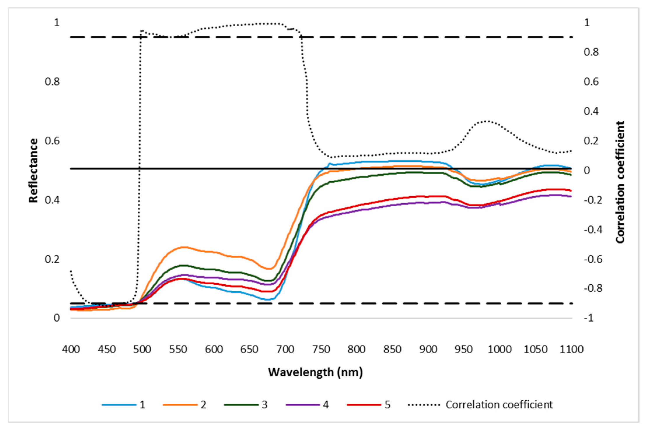
An aphid is a sucking insect pest. It affects the green and non-green pigments of the plant that is clearly visible in the 400–700 nm spectral region. The ground-measured reflectance for healthy mustard crop plants remains more in the blue (431–498 nm) and near infrared (750–1100 nm) spectral regions. The reflectance was more compared to the infested plants in the red (560–700 nm) region (Figure 3). The reflectance data were highly correlated to AISG within the region 490–720 nm.
Figure 3.
Spectral reflectance of different AISGs of mustard leaves and their correlation coefficient. The significant level of correlation coefficient at x = 0.01 was indicated by the solid horizontal line. 1, 2, 3, 4, and 5 are different severity grades of aphid-infested mustard crop (from no infestation to high severe).The values of first derivative reflectance data indicated two different peaks, first at 502 nm (blue) and second at 699 nm (red) and had three different lower lobes at 572 nm (green), 612 nm, and 662 nm (red) spectral regions. The correlation coefficient between the first derivative and the respective AISG showed that as the first derivative decreases, the AISG increases significantly (Figure 4). The first derivative showed that the maximum change in the slope of the reflectance at 502 nm, 572 nm, 612 nm, and 662 nm may be due to deviation in anthocyanin and chlorophyll contents, respectively, between healthy and mustard aphid-infested crops.

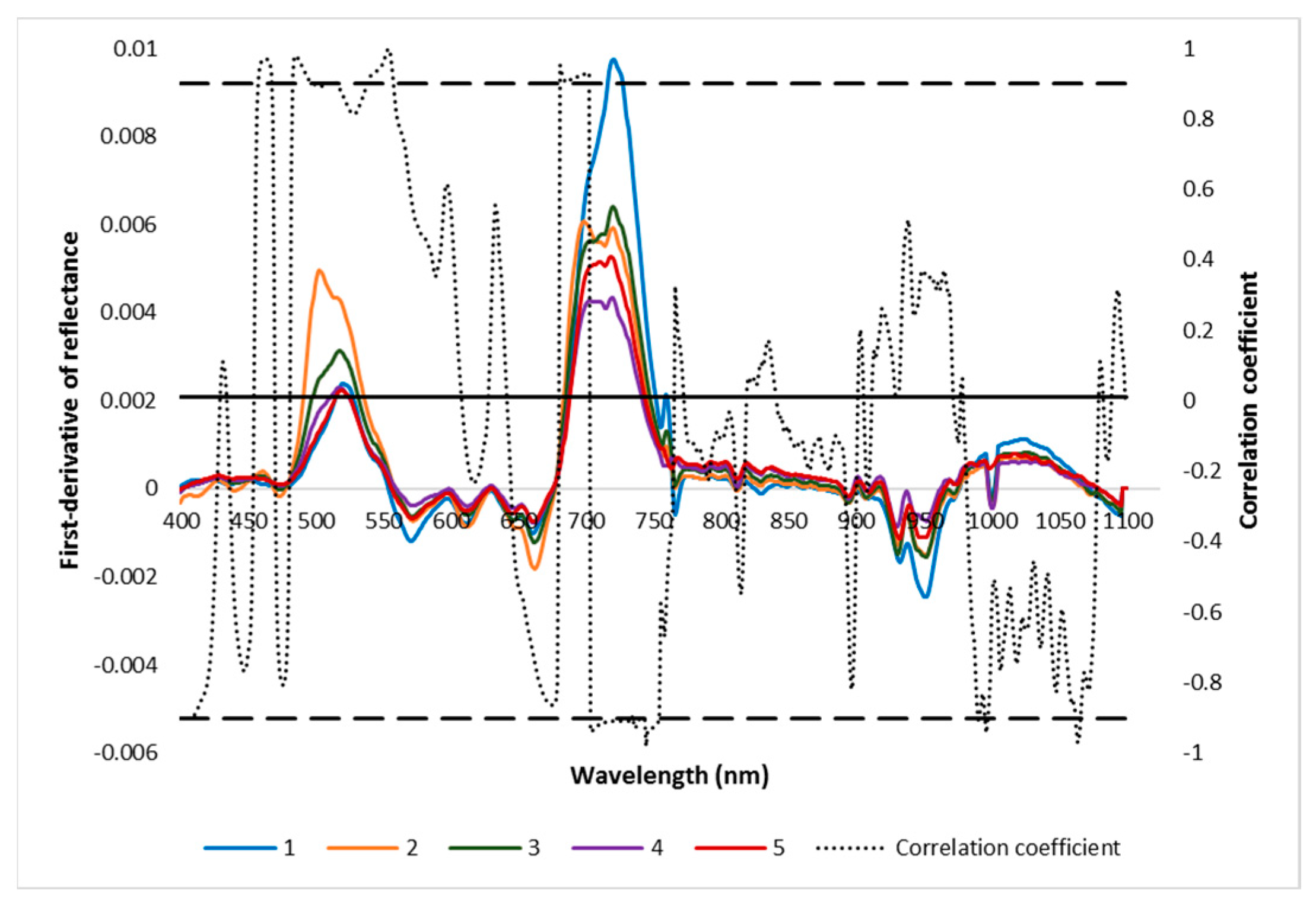
Figure 4.
First derivative of reflectance of different AISGs of mustard leaves and their correlation coefficient. The significant level of correlation coefficient at x = 0.01 was indicated by the solid horizontal line. 1, 2, 3, 4, and 5 are different severity grades of aphid-infested mustard crop (from no infestation to high severe).

The second derivative shows the rate of change in the slope of the reflectance curve (Figure 5). The second derivative values of reflectance significantly increased with an increase in AISG in the 477–489 nm and 690–715 nm spectral regions.
3.2. Biochemical Analysis of Mustard Crop
The analyzed plant samples showed that the total anthocyanin content (analyzed with dry weight method) in the aphid-infested plants was significantly (p < 0.05) lower at the AISG of grade 3 (40%), grade 4 (25%), and grade 5 (21%) as compared to grade 1. Chlorophyll a, b, and total chlorophyll were significantly lower at different severity levels, viz., grade 2/3 (96%, 85% and 93%), grade 4 (96%, 86% and 93%), and grade 5 (55%, 44% and 52%), as compared to healthy crops. Total carotenoids were also lower at grade 2/3 (78%), grade 4 (76%), and grade 5 (11%). The variation in biochemical content at different aphid severity levels as compared to the initial infested stage is due to the internal plant response mechanism to build resistance against aphid infestation.
3.3. Sensitive Spectral Regions and Bands for AISG
Field-based reflectance of mustard crop and its first and second derivatives was found to be significantly correlated with AISG at four different spectral regions. The spectral regions 483–487 nm, 509–515 nm, 690–714 nm, and 719–723 nm (Figure 6, Table 4) showed significant correlation with AISG (level of significance: 99%) for reflectance and derivatives (1st and 2nd) that were identified to discriminate healthy and aphid-infested crops.
Further, PCA and PLSR analysis was done for the healthy and aphid-infested crops for the selection of dominant spectral bands. The “PC loadings/factor loading weight” can be used to select sensitive bands that are extremely correlated to each PC/factor. Loading weights of the first three PCs/factors were used to select sensitive bands in the entire spectral range (400–1000 nm). The spectral bands corresponding to peak and lower lobes at these particular PCs were chosen as sensitive spectral bands (Figure 7a,b). The four spectral bands were identified in each PCA (500 nm, 679 nm, 746 nm, 979 nm) and PLSR (491 nm, 679 nm, 746 nm, 979 nm) that discriminated AISG levels (Table 3). Such a reduced number of predictors (spectral bands) would support sinking the time required to obtain and process each available spectral band of the satellite data.
3.4. Regression Model
Average reflectance (R) and three indices (RSI, DSI, and NDSI) of sensitive spectral regions and absolute reflectance (r) of sensitive specific spectral bands were found to investigate the AISG using different regression methods (Table 4). All factors were significantly related to AISG and DSI, with absolute reflectance being the most sensitive one. The linear regression (Linear, Interactions, and Robust), Coarse tree regression, Support vector machine (Coarse Gaussian, Cubic, Gaussian, Fine, Linear, Medium Gaussian, and Quadratic), Ensemble Tree (Boosted Trees), and Gaussian Process regression (Matern 5/2, Rational Quadratic, and Squared Exponential) were not significantly correlated with AISG. Stepwise linear and Ensemble (Bagged Trees) regressions were sensitive to all the factors and found that the stepwise linear regression was most sensitive with RSI (RMSE = 0.69 and R square = 0.67) (Table 4). The model using RSI had great potential to evaluate the AISG variety at a plant level.
3.5. PCR for Detection of AISG of Mustard Crop
The PCR results showed that the first PC, second PC, and third PC explained 72%, 21%, and 6% of the total variance of the original hyperspectral dataset (Table 5). It indicates the cumulative reliability of the first three PCs that could explain 99% of the total variation; they could be capable of representing all variables for the characterization of AISGs of the mustard crops. The PCA result is commonly interpreted by visualization of its PC score (Figure 8a). The healthy and different AISGs of mustard crops are scattered separately in the three-dimension curve (Figure 8a). Consequently, the top three PCs can be taken as the predictors and the remaining can be removed from further examination. The top three PCs were used as the independent variable to develop the regression model for the estimation of the AISGs. The scatter plots of observed vs. predicted AISG for the training and testing datasets are presented in Figure 9a. The coefficient of determination (R2) calculated between predicted and observed AISGs for training and testing data was approximately 0.56 and 0.65, respectively. In the meantime, low RMSEs of 0.78 and 0.72 were found for the training and testing data, respectively. The PCR method was used effectively to determine the spectral information of aphid-infested plants [49]. However, the high coefficient of determination (R2) and low prediction error were obtained for both training and testing data, and results advised that the AISG of the mustard crops was explained by the first three PCs.
3.6. PLSR for ASIG of Mustard Crop
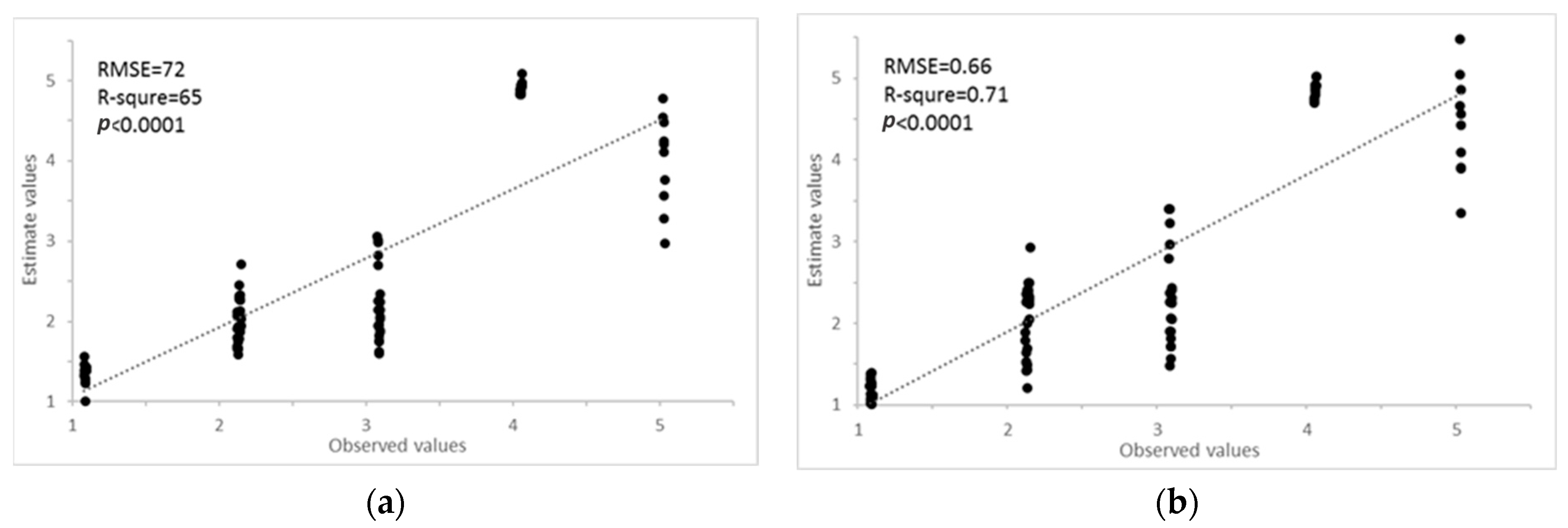
PLSR was computed using the training data. Three factors were able to explain 99.53% of the model variance and 99.51% of the variance for forecast (Table 5). The seven factors of the PLS model for the training dataset were applied for the prediction of AISG of the testing dataset. The result of PLS is usually interpreted by visualization of its factor score (Figure 8b). It can be found that healthy and different AISGs of mustard crop are distributed separately in three dimension areas. Hence, the top three factors can be regarded as the predictors and the remaining can be removed from further investigation. The correlation coefficient between observed and predicted values for calibration and testing of samples were 0.62 and 0.71, respectively. The RMSE of calibration and validation were 0.72 and 0.66, respectively (Figure 9b). Clearly, the AISGs were more precise according to RMSE values compared to the other methods.
In this research, the high coefficient of determination (R2 = 0.71) and low prediction errors (RMSE = 0.66) were obtained with PLS regression for the calibration and validation dataset and results advised that the AISG of the mustard crops was well-explained by the first three factors (Figure 8b, Table 6). A similar strategy was adopted by [12,50] for the prediction of protein content and grain yield using hyperspectral reflectance data.
4. Discussion
In our study, various regression models, multivariate, and multidimensional statistical methods were examined to evaluate their performances in the assessment of AISGs of mustard crops using remotely-sensed hyperspectral reflectance data. Average reflectance, absolute reflectance, and generated vegetation indices (estimated from average reflectance of selected spectral regions) were used in regression models as input variables and the optimal spectral regions and specific bands that were sensitive to AISGs were selected using different feature selection methods like sensitivity analysis, principal component analysis, and partial least square regression. Hyperspectral reflectance from 400–1100 nm was used in multivariate, multidimensional statistical methods to predict AISGs of mustard crops.
The primary cause of variation in visible region of the spectrum is the deviation in the leaf chlorophyll ‘a’ (96.4%), chlorophyll ‘b’ (85.2%), carotenoids (78%), and anthocyanin (39.8%) between healthy and low levels of severity of aphid infestation in crops, whereas deviation in chlorophyll + nitrogen + cell structure, cell structure, and available water content was responsible for alterations in reflectance values of the red edge, NIR, and SWIR regions, respectively. [51] also reported that the insect pest would pierce the leaf and suck out leaf juice, which caused a drop in chlorophyll and leaf water content in wheat crops.
Although the reflectance data were highly correlated to AISG within the region 490–720 nm, several authors [52,53,54] reported that the variation in the spectral region 400–700 nm is due to pest infestation. The variation in these green and non-green pigment regions is quite evident, and the ground data also showed the same. The first derivative showed maximum variation in the slope at 502 nm, 572 nm, 612 nm, and 662 nm between healthy and aphid-infested mustard crops. In addition, the second derivative values of reflectance significantly increased with an increase in AISG in the 477–489 nm and 690–715 nm spectral regions. This showed that the mustard aphid infestation produced a deviation in green (chlorophyll a and b) and non-green (carotenoids and anthocyanin) pigments between healthy and infested crops. Earlier reports indicate similar changes in phytocompounds with relation to a hyperspectral anomaly between healthy and disease-infested wheat crops [30,55], but are rare [56] in insect herbivory. [29] showed that aphid infestation in mustard crops adversely affects biochemical properties such as carbohydrates, lipids, nitrogen, and protein ranks of several parts of plants such as leaf, stem, inflorescence, and seeds at different growth stages due to the sucking of different biochemical content by aphids. This led to an effect on the leaf chlorophyll content, as observed from the lab-based analysis. However, the spectral range 690–715 nm is sensitive to discriminate healthy and different AISGs in the mustard crop. Therefore, it is possible to detect different AISGs using the hyperspectral data. The variation in biochemical content at different aphid severity levels as compared to the initial infested stage is due to the internal plant response mechanism to build resistance against aphid infestation. [51] also reported similar results, which showed that physical and chemical barriers play a pivotal role in generating resistance against aphid infestation.
PCA and PLSR were successfully used to select the highly sensitive bands to AISGs of mustard crops. Several researchers, [44,45] used these methods to select optimal variables or spectral bands for better prediction accuracy. The four spectral bands (500 nm, 679 nm, 746 nm, 979 nm) were identified to develop the prediction models and the selected spectral bands were neither associated to the known water absorption spectral bands at 970 nm, 1200 nm, 1400 nm, 1450 nm, and 1940 nm nor with leaf pigment absorption spectral bands 430 nm, 460 nm, 640 nm, and 660 nm [52]. It was observed that the spectral bands of 500 nm and 679 nm were positioned in the green and red regions that were poorly absorbed by chlorophyll and other pigments, while the bands 746 nm and 979 nm were located after the red edge region, where vegetation spectral data are sensitive to pest infestation.
All the evaluating errors of the tested prototypes (PCR and PLSR) were significantly good for the detection of AISG, excluding some models. Ref. [57] reported that the high covariance and redundancy in spectroscopic/hyperspectral data affected the precision of prediction. However, low R2 and high RMSE of PCR were found for both calibration and validation datasets compared to PLS, and results recommended that AISG was probably affected by other factors not explained by the top three PCs. [58] reported that achieving a high level of accuracy with PCR was difficult because PCR accepted independent variables (spectral bands) without considering the dependent variable. Therefore, PLS techniques are the ideal techniques for removing the variable (spectral bands). PLSR was found to be the most sensitive, with an RMSE of 0.72 with R2 0.62 for training and an RMSE of 0.66 with R2 0.71 for validation compared to other models. The findings of [12,50] corroborated with our results. Therefore, prediction with PLSR was most sensitive for the detection of AISG of mustard crops.
5. Conclusions
Crops losses due to insect pests have previously been assessed by measuring reflectance at the leaf and canopy levels. The present findings demonstrated that ground measured reflectance and transmitted energy curves varied in magnitude and curvature for healthy and aphid-infested crop plants. In this study, we found that four sensitive spectral regions (483–487 nm, 509–515 nm, 690–714 nm, and 719–723 nm) and three specific spectral bands (500 nm, 679 nm, 746 nm, and 979 nm) were significantly correlated with AISG. Spectral region (483–487 nm and 509–515 nm) and spectral bands (500 nm, 679 nm, and 687 nm) are mainly related to chlorophyll content and non-green pigments. Therefore, the remaining spectral regions (690–714 nm and 719–723 nm) and bands (746 nm and 979 nm) are most sensitive to AISGs and have the ability to discriminate aphid-infested mustard crops from healthy ones.
The three spectral indices, DSI, RSI, and NDSI, were calculated using leaf reflectance of four sensitive spectral regions (483–487 nm, 509–515 nm, 690–714 nm, and 719–723 nm) that were strongly related to AISG. The regression models for evaluating the AISG of the mustard crops were tested using the average reflectance, values of indices, and absolute reflectance. It was found that the stepwise linear regression is most sensitive with RSI (RMSE = 0.69 and R square = 0.67). The model using RSI had shown great potential to evaluate the AISG at a plant level.
Among all the performances of regression analysis, using PLSR to estimate AISG of the mustard crops was found to be superior to reflectance, indices, and PCR. Therefore, PLSR can be used to discriminate the different AISGs of the mustard crops from hyperspectral data. The prediction errors showed RMSE of 0.72 (R square = 0.62) and 0.66 (R square = 0.71) for testing and validating datasets, respectively. The present study showed that different AISGs can be segregated from healthy mustard crops using hyperspectral data. Future studies will be able to utilize this method and identify sensitive spectral regions to discriminate healthy and aphid-infested crops using ground, aerial, and satellite-based hyperspectral and multispectral data from sensors.
Author Contributions
Conceptualization, K.K.S., R.N. and A.K.K.; methodology, K.K.S. and R.N.; software, K.K.S. and R.N.; validation, K.K.S., R.N. and A.B.; formal analysis, K.K.S. and R.N.; investigation, A.B. and R.N.; resources, R.N. and A.B. and B.K.B.; data curation, A.K.K., K.K.S., A.B., A.K. and R.N.; writing—original draft preparation, K.K.S.; writing—review and editing, A.B, R.N., S.C. and K.K.S.; visualization, A.B.; supervision, B.K.B. and S.C.; project administration, A.B. and R.N; funding acquisition, A.B. and A.K.K. All authors have read and agreed to the published version of the manuscript.
Funding
The work was funded by the Space Applications Centre (SAC) a major centre of Indian Space Research Organization (ISRO), Ahmedabad, India.
Data Availability Statement
Data is unavailable due to privacy or ethical restrictions.
Acknowledgments
We acknowledge the Space Technology Utilization for Food Security, Agricultural Assessment and Monitoring (SUFALAM) programme of the Space Applications Centre, Indian Space Research Organization, Ahmedabad for designing this study and providing the necessary support. We would also like to thanks Aparna Chattopadhyay for improving the language of the paper and Vijay Paul, Division of Plant Physiology, IARI pusa, for providing resources (biochemical analysis).
Conflicts of Interest
The authors declare no conflict of interest.
References
- DAC. Directorate of Economics and Statistics, Department of Agriculture and Corporation. 2015. Available online: https://eands.dacnet.nic.in/ (accessed on 15 May 2022).
- Kumar, D.; Kalita, P. Reducing Postharvest Losses during Storage of Grain Crops to Strengthen Food Security in Developing Countries. Foods 2017, 6, 8. [Google Scholar] [CrossRef] [PubMed]
- Jeger, M.; Beresford, R.; Bock, C. Global challenges facing plant pathology: Multidisciplinary approaches to meet the food security and environmental challenges in the mid-twenty-first century. CABI Agric. Biosci. 2021, 2, 20. [Google Scholar] [CrossRef]
- West, J.S.; Bravo, C.; Oberit, R.; Lemaire, D.; Moshou, D.; McCartney, H.A. The potential of optical canopy measurement for targeted control of field crop diseases. Annu. Rev. Phytopathol. 2003, 41, 593–614. [Google Scholar] [CrossRef] [PubMed]
- Government of India, Ministry of Agriculture. 2019–2020. Available online: https://www.sopa.org/india-oilseeds-area-production-and-productivity (accessed on 15 May 2022).
- FAO (Food and Agriculture Organization). FAOSTAT, Crop and Livestock Products, United Nations. 2022. Available online: https://www.fao.org/faostat/en/#data/QCL (accessed on 14 March 2022).
- Patel, S.R.; Awasthi, A.K.; Tomar, R.K.S. Assessment of yield losses in mustard (Brassica juncea L.) due to mustard aphid (Lipaphis erysimi Kalt.) under different thermal environments in eastern central India. Appl. Ecol. Environ. Res. 2004, 2, 1–15. [Google Scholar] [CrossRef]
- Shylesha, A.N.; Thakur, A.N.S.; Pathak, K.A.; Rao, K.R.; Saikia, K.; Surose, S.; Kodandaram, N.H.; Kalaishekar, A. Integrated Management of Insect Pest of Crops in North Eastern Hill Region; Technical Bulletin No. 19; ICAR RC for NEH Region: Umiam, Meghalaya, India, 2006; Volume 50. [Google Scholar]
- Kular, J.S.; Kumar, S. Quantification of avoidable yield losses in oilseed Brassica caused by insect pests. J. Plant Prot. Res. 2011, 51, 38–43. [Google Scholar] [CrossRef]
- Raikes, C.; Burpee, L.L. Use of multispectral radiometry for assessment of Rhizoctonia blight in creeping bentgrass. Phytopathology 1998, 88, 446–449. [Google Scholar] [CrossRef] [PubMed]
- Singh, P.; Sinhal, V.K. Effect of Aphid infestation on the Biochemical Constituents of Mustard (Brassica juncea) plant. J. Phytol. 2011, 3, 28–33. [Google Scholar]
- Terentev, A.; Dolzhenko, V.; Fedotov, A.; Eremenko, D. Current state of hyperspectral remote sensing for early plant disease detection: A review. Sensors 2022, 22, 757. [Google Scholar] [CrossRef]
- Kumar, A.; Bhattacharya, B.K.; Kumar, V.; Jain, A.K.; Mishra, A.K.; Chattopadhyay, C. Epidemiology and forecasting of insect-pests and diseases for value-added agro-advisory. Mausam 2016, 67, 267–276. [Google Scholar] [CrossRef]
- Jackson, H.R.; Wallen, V.R. Microdensitometer measurements of sequential aerial photographs of field beans infected with bacterial blight. Phytopathology 1975, 65, 961–968. [Google Scholar] [CrossRef]
- Colwell, R.N. Determining the prevalence of certain cereal diseases by means of aerial photography. Hilgardia 1956, 26, 223–286. [Google Scholar] [CrossRef]
- Jackson, R.D. Remote sensing of biotic and abiotic plant stress. Annu. Rev. Phytopathol. 1986, 24, 265–287. [Google Scholar] [CrossRef]
- Nilsson, H.E. Remote sensing and image analysis in plant pathology. Annu. Rev. Phytopathol. 1995, 33, 489–527. [Google Scholar] [CrossRef] [PubMed]
- Mirik, M.; Michels, G.J., Jr.; Kassymzhanova-Mirik, S.; Elliott, N.C. Reflectance characteristics of Russian wheat aphid (Hemiptera: Aphididae) stress and abundance in winter wheat. Comput. Electron. Agric. 2007, 57, 123–134. [Google Scholar] [CrossRef]
- Mirik, M.; Michels, G.J., Jr.; Kassymzhanova-Mirik, S.; Elliott, N.C.; Catana, V.; Jones, D.B.; Bowling, R. Using digital image analysis and spectral reflectance data to quantify damage by greenbug (Hemitera: Aphididae) in winter wheat. Comput. Electron. Agric. 2006, 51, 86–98. [Google Scholar] [CrossRef]
- Huang, J.F.; Apan, A. Detection of sclerotinia rot disease on celery using hyperspectral data and partial least squares regression. J. Spat. Sci. 2006, 52, 129–142. [Google Scholar] [CrossRef]
- Govender, M.; Chetty, K.; Bulcock, H. A review of hyperspectral remote sensing and its application in vegetation and water resource studies. Water Sci. 2007, 33, 145–152. [Google Scholar] [CrossRef]
- Singh, D.; Sao, R.; Singh, K.P. A remote sensing assessment of pest infestation on sorghum. Adv. Space Res. 2007, 39, 155–163. [Google Scholar] [CrossRef]
- Card, D.H.; Peterson, D.L.; Matson, P.A. Prediction of leaf chemistry by the use of visible and near infrared reflectance spectroscopy. Remote Sens. Environ. 1988, 26, 123–147. [Google Scholar] [CrossRef]
- Yoder, B.J.; Pettigrew-Crosby, R.E. Predicting nitrogen and chlorophyll content and concentrations from reflectance spectra (400~2500 nm) at leaf and canopy scales. Remote Sens. Environ. 1995, 53, 199–211. [Google Scholar] [CrossRef]
- Liu, Z.-Y.; Huang, J.F.; Shi, J.J.; Tao, R.X.; Zhou, W.; Zhang, L.L. Characterizing and estimating rice brown spot disease severity using stepwise regression, principal component regression and partial least-square regression. J. Zhejiang Univ. Sci. B 2007, 8, 738–744. [Google Scholar] [CrossRef] [PubMed]
- Golhani, K.; Balasundram, S.K.; Vadamalai, G.; Pradhan, B. A review of neural networks in plant disease detection using hyperspectral data. Inf. Process. Agric. 2018, 5, 354–371. [Google Scholar] [CrossRef]
- Kimes, D.S.; Nelson, R.F.; Manry, M.T.; Fung, A.K. Attributes of neural networks for extracting continuous vegetation parameters from optical and radar measurements. Int. J. Remote Sens. 1998, 19, 2639–2663. [Google Scholar] [CrossRef]
- Muhammed, H.H.; Larsolle, A. Feature vector based analysis of hyperspectral crop reflectance data for discrimination and quantification of fungal disease severity in wheat. Biosyst. Eng. 2003, 86, 125–134. [Google Scholar] [CrossRef]
- Lu, J.; Ehsani, R.; Shi, Y.; de Castro, A.I.; Wang, S. Detection of multi-tomato leaf diseases (late blight, target and bacterial spots) in different stages by using a spectral-based sensor. Sci. Rep. 2018, 8, 2793. [Google Scholar] [CrossRef] [PubMed]
- Whetton, R.L.; Hassall, K.L.; Waine, T.W.; Mouazen, A.M. Hyperspectral measurements of yellow rust and fusarium head blight in cereal crops: Part 1: Laboratory study. Biosyst. Eng. 2018, 166, 101–115. [Google Scholar] [CrossRef]
- Kumar, J.; Vashisth, A.; Sehgal, V.K.; Gupta, V.K. Assessment of aphid infestation in Mustard by Hyperspectral remote sensing. J. Indian Soc. Remote Sens. 2013, 41, 83–90. [Google Scholar] [CrossRef]
- Koirala, S. Mustard Aphid and Crop Production. Int. J. Appl. Sci. Biotechnol. 2020, 8, 310–317. [Google Scholar] [CrossRef]
- Hiscox, J.D.; Israelstam, G.F. A method for the extraction of chlorophyll from leaf tissue without maceration. Can. J. Bot. 1979, 57, 1332–1334. [Google Scholar] [CrossRef]
- Wellburn, A.R. The spectral determination of chlorophylls a and b, as well as total carotenoids, using various solvents with spectrophotometers of different resolution. J. Plant Physiol. 1994, 144, 307–313. [Google Scholar] [CrossRef]
- Valifard, M.; Moradshahi, A.; Kholdebarin, B. Biochemical and physiological responses of two wheat (Triticumaestivum L.) cultivars to drought stress applied at seedling stage. J. Agric. Sci. Technol. 2012, 14, 1567–1578. [Google Scholar]
- Prince, J.C. How unique is spectral signature? Remote Sens. Environ. 1994, 49, 181–186. [Google Scholar] [CrossRef]
- Thenkabail, P.S.; Enclona, E.A.; Ashton, M.S.; Van Der Meer, B. Accuracy assessments of hyperspectral waveband performance for vegetation analysis applications. Remote Sens. Environ. 2004, 91, 354–376. [Google Scholar] [CrossRef]
- Savitzky, A.; Golay, M.J.E. Smoothing and differentiation data by simplified least square procedure. Anal. Chem. 1964, 36, 1627–1638. [Google Scholar] [CrossRef]
- Ariana, D.P.; Lu, R.F. Evaluation of internal defect and surface color of whole pickles using hyperspectral imaging. J. Food Eng. 2010, 96, 583–590. [Google Scholar] [CrossRef]
- Li, J.; Li, C.; Xhao, D.; Gang, C. Non-destructive estimation of foliar pigment (chlorophyll, carotenoid and anthocyanin) content: Evaluating a semi analytical three-band model. In Hyperspectral Remote Sensing of Vegetation, 1st ed.; Thenkabail, P.S., Lyon, J.G., Eds.; CRS Press: Boca Raton, FL, USA, 2011; p. 26. [Google Scholar]
- Wu, D.; Chen, X.J.; Zhu, X.G.; Guan, X.C.; Wu, G.C. Uninformative variable elimination for improvement of successive projections algorithm on spectral multivariable selection with different calibration algorithms for the rapid and non-destructive determination of protein content in dried laver. Anal. Methods 2011, 3, 1790–1796. [Google Scholar] [CrossRef]
- Wu, D.; Chen, X.J.; Shi, P.Y.; Wang, S.H.; Feng, F.Q.; He, Y. Determination of alpha-linolenic acid and linoleic acid in edible oils using near-infrared spectroscopy improved by wavelet transform and uninformative variable elimination. Anal. Chim. Acta 2009, 634, 166–171. [Google Scholar] [CrossRef]
- Wu, D.; He, Y.; Nie, P.C.; Cao, F.; Bao, Y.D. Hybrid variable selection in visible and near-infrared spectral analysis for non-invasive quality determination of grape juice. Anal. Chim. Acta 2010, 659, 229–237. [Google Scholar] [CrossRef]
- Villa, J.; Calpe, J.; Pla, F.; Gomez, L.; Connell, J.; Marchant, J.; Calleja, J.; Mulqueen, M.; Munoz, J.; Klaren, A. The SmartSpectra Team SmartSpectra: Applying multispectral imaging to industrial environments. Real Time Imaging 2005, 11, 85–98. [Google Scholar] [CrossRef]
- Vargas, A.M.; Kim, M.S.; Tao, Y.; Lefcourt, A.M.; Chen, Y.R.; Luo, Y.; Song, Y.; Buchanan, R. Defection of fecal contamination on cantaloupes using hyperspectral fluorescence imagery. J. Food Sci. 2005, 70, 471–476. [Google Scholar] [CrossRef]
- Krishna, G.; Sahoo, R.N.; Pargal, S.; Gupta, V.K.; Sinha, P.; Bhagat, S.; Saharan, M.S.; Singh, R.; Chattopadhyay, C. Assessing wheat yellow rust disease through hyperspectral remote sensing. Int. Arch. Photogramm. Remote Sens. Spat. Inform. Sci. 2014, 8, 1413–1416. [Google Scholar] [CrossRef]
- Romain, B.; Alexis, C.; Remi, M.; Vincent, L.; Philippe, V.; Benjamin, D.; Benoit, M. In-field proximal sensing of septoria tritici blotch, stripe rust and brown rust in winter wheat by means of reflectance and textural features from multispectral imagery. Biosyst. Eng. 2020, 197, 257–269. [Google Scholar] [CrossRef]
- Fung, T.; LeDrew, E. Application of principal components analysis to change detection. Photogramm. Eng. Remote Sens. 1987, 53, 1649–1658. [Google Scholar]
- Holden, H.; LeDrew, E. Spectral discrimination of healthy and non-healthy corals base on cluster analysis, principal components analysis and derivative spectroscopy. Remote Sens Environ. 1998, 65, 217–224. [Google Scholar] [CrossRef]
- Hansen, P.M.; Jorgensen, J.R.; Thomsen, A. Predicting grain yield and protein content in winter wheat and spring barley using repeated canopy reflectance measurements and partial least squares regression. J. Agric. Sci. 2002, 139, 307–318. [Google Scholar] [CrossRef]
- Luo, J.; Huang, W.; Zhao, J.; Zhang, J.; Zhao, C.; Ma, R. Detecting Aphid Density of Winter Wheat Leaf Using Hyperspectral Measurements. IEEE J. Sel. Top. Appl. Earth Obs. Remote Sens. 2013, 6, 690–698. [Google Scholar] [CrossRef]
- Curran, P.J. Remote sensing of foliar chemistry. Remote Sens. Environ. 1956, 30, 271–278. [Google Scholar] [CrossRef]
- Galvao, L.S.; Vitorello, I.; Filho, R.A. Effects of band positioning and bandwidth on NDVI measurements of tropical savannahs. Remote Sens. Environ. 1999, 67, 181–193. [Google Scholar] [CrossRef]
- Kumar, L.; Schmidt, K.; Dury, S.; Skidmore, A. Imaging Spectrometry and Vegetation Science. In Imaging Spectrometry: Basic Principles and Prospective Applications; Van der Meer, F.D., de Jong, S.M., Eds.; Kluwer Academic Publishers: Dordrecht, The Netherlands, 2001; pp. 111–155. [Google Scholar]
- Zhang, N.; Yang, G.; Pan, Y.; Yang, X.; Chen, L.; Zhao, C. A review of advanced technologies and development for hyperspectral-based plant disease detection in the past three decades. Remote Sens. 2020, 12, 3188. [Google Scholar] [CrossRef]
- Ribeiro, L.D.P.; Klock, A.L.S.; Wordell, F.; Tramontin, M.A.; Trapp, M.A.; Mithöfer, A.; Nansen, C. Hyperspectral imaging to characterize plant-plant communication in response to insect herbivory. Plant Methods 2018, 14, 54. [Google Scholar] [CrossRef]
- Thenkabail, P.S.; Smith, R.B.; Pauw, E.D. Hyperspectral vegetation indices and their relationships with agricultural crop characteristics. Remote Sens. Environ. 2000, 71, 158–182. [Google Scholar] [CrossRef]
- Monteiro, S.T.; Minekawa, Y.; Kosugi, Y.; Akazaw, T.; Oda, K. Prediction of sweetness and amino acid content in soybean crops from hyperspectral imagery. ISPRS J. Photogramm. Remote Sens. 2007, 62, 2–12. [Google Scholar] [CrossRef]
Figure 1.
Study area.

Figure 2.
Flow of methodology.

Figure 5.
2nd derivative of reflectance of different AISGs of mustard leaves and their correlation coefficient. The significant level of correlation coefficient at x= 0.01 was indicated by the solid horizontal line. 1, 2, 3, 4, and 5 are different severity grades of aphid-infested mustard crop (from no infestation to high severe).

Figure 6.
The sensitive spectral regions for detecting of AISG of mustard plant. The spectral region covered by a solid lines indicated a significant correlation between spectral reflectance (red), 1st derivative (purple) and 2nd derivative (black) and AISGs. Overlapping sensitive regions (green color) from reflectance, first derivative, and second derivative (Table 3).

Figure 7.
(a) Loading weight of the first three PCs from PCA on reflectance of mustard plant. (b) Loading weight of the first three factors from the PLSR of mustard plant.
Figure 7.
(a) Loading weight of the first three PCs from PCA on reflectance of mustard plant. (b) Loading weight of the first three factors from the PLSR of mustard plant.

Figure 8.
(a) Cluster plot of PC1 X PC2 X PC3 score of each healthy and aphid-infested severity grade of mustard plant. (b) Cluster plot of Factor1 X Factor2 X Factor3 score of healthy and each aphid-infested severity grade of the mustard plant. Color-coding (different aphid-infested severity grade) is blue 1, red 2, green 3, sky blue 4, and maroon 5.

Figure 9.
Regression model and their amiability of suitable for aphid infestation severity grade (AISG) using PCs (a) and factors (b). The dashed line indicated that the observed values were equal to the estimated values.
Figure 9.
Regression model and their amiability of suitable for aphid infestation severity grade (AISG) using PCs (a) and factors (b). The dashed line indicated that the observed values were equal to the estimated values.


Table 1.
Details of sample collection sites and crops.
| Site No. | Latitude and Longitude | Date of Measurement | Date of Sowing | Age of Crop/Phenological Stage |
|---|---|---|---|---|
| Site 1 | 27.20 N, 77.45 E | 5 February 2017 | 31 October 2016 | 95 days/Ripening |
| Site 2 | 27.35 N, 77.37 E | 9 February 2017 | 7 November 2016 | 92 days/Ripening |
| Site 3 | 27.25 N, 77.46 E | 18 January 2017 | 7 November 2016 | 75 days/Ripening |
| Site 4 | 27.48 N, 77.26 E | 5 December 2017 | 21 October 2016 | 45 days/Inflorescence emergence |
| Site 5 | 27.50 N, 77.15 E | 31 January 2018 | 30 November 2017 | 60 days/Flowering |
| Site 6 | 27.08 N, 77.19 E | 22 January 2018 | 22 October 2017 | 60 days/Flowering and ripening |
| Site 7 | 27.23 N, 77.47 E | 31 January 2018 | 26 October 2017 | 95 days/Ripening |
| Site 8 | 27.47 N, 77.28 E | 5 December 2017 | 21 October 2016 | 45 days/Inflorescence emergence |
Table 2.
Aphid infestation severity grade (AISG) according to plant part damage characteristics.
| Severity Grade | Infestation Severity | Aphids/Plant | Plant Part Damage Characteristics |
|---|---|---|---|
| 1 | No infestation (Healthy)  | Nil | No aphid infestation plant manifests excellent growth. Albeit a single aphid was found on tender parts of the plant viewed as infested |
| 2 | Initial | 0–25 | Yellowing of older leaves |
| 25–50 | Average growth of the plant, leaf form got curls, and yellowing of a couple of leaves average flowering and pod setting on virtually all the twigs. A few aphid colonies were found on a couple of twigs and topical shoots | ||
| 3 | Low | 25–50 | Less than average growth, yellowing and curling of leaves on few twigs. Plant appears slight stunted with a smaller number of flowering and little pod setting |
| 50–75 | Plant growth normal, leaf yellowing and shape became curls of older leaves, normal flowering and pod setting on almost all the branches | ||
| 4 | Moderate | 50–75 | Plant growth very poor, large number of curling and yellowing leaves. Plant appears moderate stunted, minimal flowering, and only a few pods formed |
| 75–100 | Growth less than average. Plant appears slightly stunted with yellowing and curling of young and older leaves | ||
| 5 | Severe | 75–100 | Plant growth was very weakened and stunted. Despite the abundant number of curling and yellowing of the leaves, only a few flowerings and pods setting. Outnumbering aphid population on plants. Maximum of stems and leaves surface are hidden with sooty mold, no flowering, no pod formation |
| >100 | Heavy infestation damaged plant growth becomes a virtually stunted condition, curling leaf manifest crackling, and yellowing of virtually all the leaves. No flowering and pod development at all and plant ample of aphid. |
Source: Plant part damage characteristics described by Ref. [32].
Table 3.
Regression model and their amiability of suitable for aphid infestation severity grade (AISG) using average reflectance, all indices, and absolute reflectance.
Table 3.
Regression model and their amiability of suitable for aphid infestation severity grade (AISG) using average reflectance, all indices, and absolute reflectance.
| Model | Method | Evaluation Factor | Input Factors | ||||
|---|---|---|---|---|---|---|---|
| R | RSI | DSI | NDSI | r | |||
| Linear Regression Model | Linear, Interactions and Robust | Not applicable | |||||
| Stepwise Linear | RMSE | 0.74 | 0.69 | 0.83 | 0.79 | 0.84 | |
| R Square | 0.62 | 0.67 | 0.53 | 0.57 | 0.51 | ||
| Regression Tree | Fine tree | RMSE | 1.2 | 1.2 | 1.20 | 1.20 | 1.2 |
| R Square | 0 | 0 | 0 | 0 | 0 | ||
| Medium tree | RMSE | 1.2 | 1.2 | 1.20 | 1.20 | 1.2 | |
| R Square | 0 | 0 | 0 | 0 | 0 | ||
| Coarse tree | RMSE | 1.2 | 1.2 | 1.20 | 1.20 | 1.2 | |
| R Square | 0 | 0 | 0 | 0 | 0 | ||
| Support Vector machine | Linear, Quadratic, Cubic, Fine Gaussian, Medium Gaussian and Coarse Gaussian | Not applicable | |||||
| Ensemble Tree | Boosted Trees | RMSE | 1.2 | 1.2 | 1.21 | 1.21 | |
| R Square | 0.01 | 0 | 0 | 0 | |||
| Bagged Trees | RMSE | 0.88 | 0.85 | 0.92 | 0.84 | ||
| R Square | 0.46 | 0.49 | 0.42 | 0.51 | |||
| Gaussian Process regression | Squared Exponential GPR | Not applicable | |||||
| Matern 5/2 GPR | RMSE | 1.2 | 1.2 | 1.2 | 1.2 | 1.2 | |
| R Square | 0 | 0 | 0 | 0 | 0 | ||
| Exponential GPR | RMSE | 1.79 | 1.78 | 1.34 | 1.63 | 1.5 | |
| R Square | 0 | 0 | 0 | 0 | 0.01 | ||
| Rational Quadratic GPR | Not applicable | ||||||
Note: R = Average reflectance, DSI = Difference spectral indices, RSI = Ratio spectral indices, NDSI = normalized difference spectral indices, r = absolute reflectance, RMSE = root mean square error.
Table 4.
List of sensitive spectral regions and specific bands for detection of different AISG.
| Methods | Spectral Region/Band |
|---|---|
| Reflectance | 431–469, 498–723 |
| 1st Derivative | 400–409, 457–467, 483–500, 509–516, 538–557, 681–754, 1062–1065 |
| 2nd Derivative | 420–425, 437–442, 454–462, 466–474, 477–489, 509–515, 519–523, 690–714, 1089–1091 |
| Common | 483–487, 509–515, 690–714, 719–723 |
| PCA | 500, 679, 746, 979 |
| PLSR | 491, 679, 746, 979 |
| Common | 500, 679, 746, 979 |
Table 5.
Percentage of variation accounted by principal component analysis (PCA) and partial least square (PLS) (training dataset).
Table 5.
Percentage of variation accounted by principal component analysis (PCA) and partial least square (PLS) (training dataset).
| PCS/Factors | PLS | PCA | ||||||
|---|---|---|---|---|---|---|---|---|
| Model Effect (%) | Prediction (%) | Model Effect (%) | Prediction (%) | |||||
| Individual | Cumulative | Individual | Cumulative | Individual | Cumulative | Individual | Cumulative | |
| 1 | 88.41 | 88.41 | 88.22 | 88.22 | 85.98 | 85.98 | 85.79 | 85.79 |
| 2 | 10.02 | 98.43 | 10.40 | 98.40 | 12.26 | 98.24 | 12.42 | 98.21 |
| 3 | 1.10 | 99.53 | 1.12 | 99.52 | 1.29 | 99.53 | 1.30 | 99.51 |
| 4 | 0.16 | 99.69 | 0.14 | 99.68 | 0.14 | 99.67 | 0.14 | 99.65 |
| 5 | 0.12 | 99.81 | 0.12 | 99.80 | 0.10 | 99.77 | 0.11 | 99.76 |
| 6 | 0.09 | 99.89 | 0.09 | 99.89 | 0.07 | 99.84 | 0.07 | 99.83 |
| 7 | 0.05 | 99.94 | 0.03 | 99.93 | 0.07 | 99.91 | 0.07 | 99.90 |
Table 6.
Goodness of PCR and PLSR to fit for aphid infestation severity grade (AISG).
| Evaluating Factors | PCA | PLSR | ||
|---|---|---|---|---|
| Training | Validation | Training | Validation | |
| RMSE | 0.78 | 0.72 | 0.72 | 0.66 |
| R square | 0.56 | 0.65 | 0.62 | 0.71 |
Disclaimer/Publisher’s Note: The statements, opinions and data contained in all publications are solely those of the individual author(s) and contributor(s) and not of MDPI and/or the editor(s). MDPI and/or the editor(s) disclaim responsibility for any injury to people or property resulting from any ideas, methods, instructions or products referred to in the content. |
© 2023 by the authors. Licensee MDPI, Basel, Switzerland. This article is an open access article distributed under the terms and conditions of the Creative Commons Attribution (CC BY) license (https://creativecommons.org/licenses/by/4.0/).
Share and Cite
MDPI and ACS Style
Shukla, K.K.; Nigam, R.; Birah, A.; Kanojia, A.K.; Kumar, A.; Bhattacharya, B.K.; Chander, S. Detection of Aphid-Infested Mustard Crop Using Ground Spectroscopy. Remote Sens. 2024, 16, 47. https://doi.org/10.3390/rs16010047
AMA Style
Shukla KK, Nigam R, Birah A, Kanojia AK, Kumar A, Bhattacharya BK, Chander S. Detection of Aphid-Infested Mustard Crop Using Ground Spectroscopy. Remote Sensing. 2024; 16(1):47. https://doi.org/10.3390/rs16010047
Chicago/Turabian StyleShukla, Karunesh K., Rahul Nigam, Ajanta Birah, A. K. Kanojia, Anoop Kumar, Bimal K. Bhattacharya, and Subhash Chander. 2024. "Detection of Aphid-Infested Mustard Crop Using Ground Spectroscopy" Remote Sensing 16, no. 1: 47. https://doi.org/10.3390/rs16010047
Note that from the first issue of 2016, this journal uses article numbers instead of page numbers. See further details here.