
Investigation of the Parameters Influencing Baseline Ozone in the Western United States: A Statistical Modeling Approach
 , ,
, ,
Abstract
:1. Introduction
2. Materials and Methods
3. Results and Discussion
4. Conclusions
Author Contributions
Funding
Institutional Review Board Statement
Informed Consent Statement
Data Availability Statement
Acknowledgments
Conflicts of Interest
References
- Laurence, J.A. Ecological effects of ozone: Integrating exposure and response with ecosystem dynamics and function. Environ. Sci. Policy 1998, 1, 179–184. [Google Scholar] [CrossRef]
- Lippmann, M. Health effects of tropospheric ozone. Environ. Sci. Technol. 1991, 25, 1954–1962. [Google Scholar] [CrossRef]
- Zhang, J.; Wei, Y.; Fang, Z. Ozone Pollution: A Major Health Hazard Worldwide. Front. Immunol. 2019, 10, 2518. [Google Scholar] [CrossRef] [PubMed] [Green Version]
- U.S. EPA. NAAQS Table. Criteria Air Pollutants. 2016. Available online: https://www.epa.gov/criteria-air-pollutants/naaqs-table (accessed on 30 June 2022).
- Jaffe, D.A.; Ninneman, M.; Chan, H.C. NOx and O3 Trends at U.S. Non-Attainment Areas for 1995–2020: Influence of COVID-19 Reductions and Wildland Fires on Policy-Relevant Concentrations. J. Geophys. Res. Atmos. 2022, 127, e2021JD036385. [Google Scholar] [CrossRef] [PubMed]
- Langford, A.O.; Alvarez, R.J., II; Brioude, J.; Fine, R.; Gustin, M.S.; Lin, M.Y.; Marchbanks, R.D.; Pierce, R.B.; Sandberg, S.P.; Senff, C.J.; et al. Entrainment of stratospheric air and Asian pollution by the convective boundary layer in the southwestern U.S. J. Geophys. Res. Atmos. 2017, 122, 1312–1337. [Google Scholar] [CrossRef]
- Nussbaumer, C.M.; Cohen, R.C. The Role of Temperature and NOx in Ozone Trends in the Los Angeles Basin. Environ. Sci. Technol. 2020, 54, 15652–15659. [Google Scholar] [CrossRef]
- Simon, H.; Reff, A.; Wells, B.; Xing, J.; Frank, N. Ozone Trends Across the United States over a Period of Decreasing NOx and VOC Emissions. Environ. Sci. Technol. 2015, 49, 186–195. [Google Scholar] [CrossRef] [Green Version]
- Jaffe, D.A.; Cooper, O.R.; Fiore, A.M.; Henderson, B.H.; Tonnesen, G.S.; Russell, A.G.; Henze, D.K.; Langford, A.O.; Lin, M.; Moore, T. Scientific assessment of background ozone over the U.S.: Implications for air quality management. Elem. Sci. Anthr. 2018, 6, 56. [Google Scholar] [CrossRef]
- Dolwick, P.; Akhtar, F.; Baker, K.R.; Possiel, N.; Simon, H.; Tonnesen, G. Comparison of background ozone estimates over the western United States based on two separate model methodologies. Atmos. Environ. 2015, 109, 282–296. [Google Scholar] [CrossRef]
- Emery, C.; Jung, J.; Downey, N.; Johnson, J.; Jimenez, M.; Yarwood, G.; Morris, R. Regional and global modeling estimates of policy relevant background ozone over the United States. Atmos. Environ. 2012, 47, 206–217. [Google Scholar] [CrossRef]
- Fiore, A.M.; Jacob, D.J.; Bey, I.; Yantosca, R.M.; Field, B.D.; Fusco, A.C.; Wilkinson, J.G. Background ozone over the United States in summer: Origin, trend, and contribution to pollution episodes. J. Geophys. Res. Earth Surf. 2002, 107, ACH-11-1–ACH 11-25. [Google Scholar] [CrossRef]
- Fiore, A.; Jacob, D.J.; Liu, H.; Yantosca, R.M.; Fairlie, T.D.; Li, Q. Variability in surface ozone background over the United States: Implications for air quality policy. J. Geophys. Res. Earth Surf. 2003, 108, ACH-19-1–ACH-19-12. [Google Scholar] [CrossRef]
- Fiore, A.M.; Oberman, J.T.; Lin, M.Y.; Zhang, L.; Clifton, O.E.; Jacob, D.J.; Naik, V.; Horowitz, L.W.; Pinto, J.P.; Milly, G.P. Estimating North American background ozone in U.S. surface air with two independent global models: Variability, uncertainties, and recommendations. Atmos. Environ. 2014, 96, 284–300. [Google Scholar] [CrossRef] [Green Version]
- Lefohn, A.S.; Emery, C.; Shadwick, D.; Wernli, H.; Jung, J.; Oltmans, S.J. Estimates of background surface ozone concentrations in the United States based on model-derived source apportionment. Atmos. Environ. 2014, 84, 275–288. [Google Scholar] [CrossRef]
- Lin, M.; Fiore, A.M.; Cooper, O.R.; Horowitz, L.W.; Langford, A.O.; Levy, H., II; Johnson, B.J.; Naik, V.; Oltmans, S.J.; Senff, C.J.; et al. Springtime high surface ozone events over the western United States: Quantifying the role of stratospheric intrusions. J. Geophys. Res. Earth Surf. 2012, 117, D00V22. [Google Scholar] [CrossRef] [Green Version]
- Miyazaki, K.; Neu, J.L.; Osterman, G.; Bowman, K. Changes in US background ozone associated with the 2011 turnaround in Chinese NOx emissions. Environ. Res. Commun. 2022, 4, 045003. [Google Scholar] [CrossRef]
- Parrish, D.D.; Ennis, C.A. Estimating background contributions and US anthropogenic enhancements to maximum ozone concentrations in the northern US. Atmos. Chem. Phys. 2019, 19, 12587–12605. [Google Scholar] [CrossRef] [Green Version]
- Parrish, D.D.; Young, L.M.; Newman, M.H.; Aikin, K.C.; Ryerson, T.B. Ozone Design Values in Southern California’s Air Basins: Temporal Evolution and U.S. Background Contribution. J. Geophys. Res. Atmos. 2017, 122, 11–166, 182. [Google Scholar] [CrossRef]
- Parrish, D.D.; Faloona, I.C.; Derwent, R.G. Observational-based assessment of contributions to maximum ozone concentrations in the western United States. J. Air Waste Manag. Assoc. 2022, 72, 434–454. [Google Scholar] [CrossRef]
- Stauffer, R.M.; Thompson, A.M.; Oltmans, S.J.; Johnson, B.J. Tropospheric ozonesonde profiles at long-term U.S. monitoring sites: 2. Links between Trinidad Head, CA, profile clusters and inland surface ozone measurements. J. Geophys. Res. Atmos. 2017, 122, 1261–1280. [Google Scholar] [CrossRef]
- Wang, H.; Jacob, D.J.; Le Sager, P.; Streets, D.G.; Park, R.J.; Gilliland, A.B.; van Donkelaar, A. Surface ozone background in the United States: Canadian and Mexican pollution influences. Atmos. Environ. 2009, 43, 1310–1319. [Google Scholar] [CrossRef] [Green Version]
- Yan, Q.; Wang, Y.; Cheng, Y.; Li, J. Summertime Clean-Background Ozone Concentrations Derived from Ozone Precursor Relationships are Lower than Previous Estimates in the Southeast United States. Environ. Sci. Technol. 2021, 55, 12852–12861. [Google Scholar] [CrossRef] [PubMed]
- Zhang, L.; Jacob, D.J.; Downey, N.V.; Wood, D.A.; Blewitt, D.; Carouge, C.C.; van Donkelaar, A.; Jones, D.B.; Murray, L.; Wang, Y. Improved estimate of the policy-relevant background ozone in the United States using the GEOS-Chem global model with 1/2° × 2/3° horizontal resolution over North America. Atmos. Environ. 2011, 45, 6769–6776. [Google Scholar] [CrossRef] [Green Version]
- Ambrose, J.L.; Reidmiller, D.R.; Jaffe, D.A. Causes of high O3 in the lower free troposphere over the Pacific Northwest as observed at the Mt. Bachelor Observatory. Atmos. Environ. 2011, 45, 5302–5315. [Google Scholar] [CrossRef]
- Zhang, L.; Jaffe, D.A. Trends and sources of ozone and sub-micron aerosols at the Mt. Bachelor Observatory (MBO) during 2004–2015. Atmos. Environ. 2017, 165, 143–154. [Google Scholar] [CrossRef]
- Jaffe, D.A.; Zhang, L. Meteorological anomalies lead to elevated O 3 in the western U.S. in June 2015. Geophys. Res. Lett. 2017, 44, 1990–1997. [Google Scholar] [CrossRef]
- Jaffe, D.A.; Fiore, A.M.; Keating, T.J. Importance of background ozone for air quality management. The Magazine for Environmental Managers, 1 November 2020; 1–5. Available online: https://pubs.awma.org/flip/EM-Nov-2020/jaffe.pdf(accessed on 19 July 2022).
- Gong, X.; Kaulfus, A.; Nair, U.; Jaffe, D.A. Quantifying O3 Impacts in Urban Areas Due to Wildfires Using a Generalized Additive Model. Environ. Sci. Technol. 2017, 51, 13216–13223. [Google Scholar] [CrossRef]
- Jaffe, D.; Prestbo, E.; Swartzendruber, P.; Weisspenzias, P.; Kato, S.; Takami, A.; Hatakeyama, S.; Kajii, Y. Export of atmospheric mercury from Asia. Atmos. Environ. 2005, 39, 3029–3038. [Google Scholar] [CrossRef]
- Baylon, P.; Jaffe, D.A.; Hall, S.R.; Ullmann, K.; Alvarado, M.J.; Lefer, B.L. Impact of Biomass Burning Plumes on Photolysis Rates and Ozone Formation at the Mount Bachelor Observatory. J. Geophys. Res. Atmos. 2018, 123, 2272–2284. [Google Scholar] [CrossRef]
- Gratz, L.E.; Jaffe, D.A.; Hee, J.R. Causes of increasing ozone and decreasing carbon monoxide in springtime at the Mt. Bachelor Observatory from 2004 to 2013. Atmos. Environ. 2015, 109, 323–330. [Google Scholar] [CrossRef]
- Zhang, L.; Jacob, D.J.; Boersma, K.F.; Jaffe, D.A.; Olson, J.R.; Bowman, K.W.; Worden, J.R.; Thompson, A.M.; Avery, M.A.; Cohen, R.C.; et al. Transpacific transport of ozone pollution and the effect of recent Asian emission increases on air quality in North America: An integrated analysis using satellite, aircraft, ozonesonde, and surface observations. Atmos. Chem. Phys. 2008, 8, 6117–6136. [Google Scholar] [CrossRef] [Green Version]
- Gaudel, A.; Cooper, O.R.; Ancellet, G.; Barret, B.; Boynard, A.; Burrows, J.P.; Clerbaux, C.; Coheur, P.-F.; Cuesta, J.; Cuevas, E.; et al. Tropospheric Ozone Assessment Report: Present-day distribution and trends of tropospheric ozone relevant to climate and global atmospheric chemistry model evaluation. Elem. Sci. Anthr. 2018, 6, 39. [Google Scholar] [CrossRef] [Green Version]
- Qu, Z.; Henze, D.K.; Cooper, O.R.; Neu, J.L. Impacts of global NOx inversions on NO2 and ozone simulations. Atmos. Chem. Phys. 2020, 20, 13109–13130. [Google Scholar] [CrossRef]
- Weiss-Penzias, P.; Jaffe, D.A.; Swartzendruber, P.; Dennison, J.B.; Chand, D.; Hafner, W.; Prestbo, E. Observations of Asian air pollution in the free troposphere at Mount Bachelor Observatory during the spring of 2004. J. Geophys. Res. Earth Surf. 2006, 111, D10304. [Google Scholar] [CrossRef]
- Chen, H.; Karion, A.; Rella, C.W.; Winderlich, J.; Gerbig, C.; Filges, A.; Newberger, T.; Sweeney, C.; Tans, P.P. Accurate measurements of carbon monoxide in humid air using the cavity ring-down spectroscopy (CRDS) technique. Atmos. Meas. Tech. 2013, 6, 1031–1040. [Google Scholar] [CrossRef] [Green Version]
- Briggs, N.L.; Jaffe, D.A.; Gao, H.; Hee, J.R.; Baylon, P.M.; Zhang, Q.; Zhou, S.; Collier, S.C.; Sampson, P.D.; Cary, R.A. Particulate Matter, Ozone, and Nitrogen Species in Aged Wildfire Plumes Observed at the Mount Bachelor Observatory. Aerosol Air Qual. Res. 2016, 16, 3075–3087. [Google Scholar] [CrossRef] [Green Version]
- Zhou, S.; Collier, S.; Jaffe, D.A.; Briggs, N.L.; Hee, J.; Sedlacek, A.J., III; Kleinman, L.; Onasch, T.B.; Zhang, Q. Regional influence of wildfires on aerosol chemistry in the western US and insights into atmospheric aging of biomass burning organic aerosol. Atmos. Chem. Phys. 2017, 17, 2477–2493. [Google Scholar] [CrossRef] [Green Version]
- Zhou, S.; Collier, S.; Jaffe, D.A.; Zhang, Q. Free tropospheric aerosols at the Mt. Bachelor Observatory: More oxidized and higher sulfate content compared to boundary layer aerosols. Atmos. Chem. Phys. 2019, 19, 1571–1585. [Google Scholar] [CrossRef] [Green Version]
- Bolton, D. The Computation of Equivalent Potential Temperature. Mon. Weather Rev. 1980, 108, 1046–1053. [Google Scholar] [CrossRef]
- Reidmiller, D.R.; Jaffe, D.A.; Fischer, E.V.; Finley, B. Nitrogen oxides in the boundary layer and free troposphere at the Mt. Bachelor Observatory. Atmos. Chem. Phys. 2010, 10, 6043–6062. [Google Scholar] [CrossRef]
- Aneja, V.P.; Businger, S.; Li, Z.; Claiborn, C.S.; Murthy, A. Ozone climatology at high elevations in the southern Appalachians. J. Geophys. Res. Earth Surf. 1991, 96, 1007. [Google Scholar] [CrossRef]
- Aneja, V.P.; Li, Z. Characterization of ozone at high elevation in the eastern United States: Trends, seasonal variations, and exposure. J. Geophys. Res. Earth Surf. 1992, 97, 9873–9888. [Google Scholar] [CrossRef]
- Lefohn, A.S.; Shadwick, D.S.; Mohnen, V.A. The characterization of ozone concentrations at a select set of high-elevation sites in the eastern United States. Environ. Pollut. 1990, 67, 147–178. [Google Scholar] [CrossRef]
- Lefohn, A.S.; Mohnen, V.A. The Characterization of Ozone, Sulfur Dioxide, and Nitrogen Dioxide for Selected Monitoring Sites in the Federal Republic of Germany. J. Air Pollut. Control Assoc. 1986, 36, 1329–1337. [Google Scholar] [CrossRef]
- Mohnen, V.A.; Hogan, A.; Coffey, P. Ozone measurements in rural areas. J. Geophys. Res. Earth Surf. 1977, 82, 5889–5895. [Google Scholar] [CrossRef] [Green Version]
- Naja, M.; Lal, S.; Chand, D. Diurnal and seasonal variabilities in surface ozone at a high altitude site Mt Abu (24.6°N, 72.7°E, 1680 m asl) in India. Atmos. Environ. 2003, 37, 4205–4215. [Google Scholar] [CrossRef]
- Wood, S.N. Generalized Additive Models: An Introduction with R; Chapman & Hall/CRC: Boca Raton, FL, USA, 2006. [Google Scholar]
- Kavassalis, S.C.; Murphy, J.G. Understanding ozone-meteorology correlations: A role for dry deposition. Geophys. Res. Lett. 2017, 44, 2922–2931. [Google Scholar] [CrossRef]
- Lu, X.; Zhang, L.; Shen, L. Meteorology and Climate Influences on Tropospheric Ozone: A Review of Natural Sources, Chemistry, and Transport Patterns. Curr. Pollut. Rep. 2019, 5, 238–260. [Google Scholar] [CrossRef] [Green Version]
- Texeira, J. AIRS/Aqua L3 Daily Standard Physical Retrieval (AIRS-only) 1 degree × 1 degree V006. Available online: https://disc.gsfc.nasa.gov/datasets/AIRS3STD_006/summary (accessed on 20 September 2022).
- Hastie, T.J.; Tibshirani, R.J. Generalized Additive Models; Chapman & Hall/CRC: Boca Raton, FL, USA, 1990. [Google Scholar]
- McClure, C.D.; Jaffe, D.A. Investigation of high ozone events due to wildfire smoke in an urban area. Atmos. Environ. 2018, 194, 146–157. [Google Scholar] [CrossRef]
- Camalier, L.; Cox, W.; Dolwick, P. The effects of meteorology on ozone in urban areas and their use in assessing ozone trends. Atmos. Environ. 2007, 41, 7127–7137. [Google Scholar] [CrossRef]
- Sun, W.; Palazoglu, A.; Singh, A.; Zhang, H.; Wang, Q.; Zhao, Z.; Cao, D. Prediction of surface ozone episodes using clusters based generalized linear mixed effects models in Houston–Galveston–Brazoria area, Texas. Atmos. Pollut. Res. 2015, 6, 245–253. [Google Scholar] [CrossRef] [Green Version]
- Jurán, S.; Edwards-Jonášová, M.; Cudlín, P.; Zapletal, M.; Šigut, L.; Grace, J.; Urban, O. Prediction of ozone effects on net ecosystem production of Norway spruce forest. iForest-Biogeos. For. 2018, 11, 743–750. [Google Scholar] [CrossRef] [Green Version]
- Cavanaugh, J.E.; Neath, A.A. The Akaike information criterion: Background, derivation, properties, application, interpretation, and refinements. WIREs Comput. Stat. 2019, 11, e1460. [Google Scholar] [CrossRef]
- CFI Team. Adjusted R-Squared. Available online: https://corporatefinanceinstitute.com/resources/knowledge/other/adjusted-r-squared/ (accessed on 1 October 2022).
- National Interagency Fire Center. Fire information: Statistics. Available online: https://www.nifc.gov/fire-information/statistics (accessed on 5 July 2022).
- Aldersley, A.; Murray, S.J.; Cornell, S.E. Global and regional analysis of climate and human drivers of wildfire. Sci. Total Environ. 2011, 409, 3472–3481. [Google Scholar] [CrossRef] [PubMed]
- Decker, Z.C.J.; Zarzana, K.J.; Coggon, M.; Min, K.-E.; Pollack, I.; Ryerson, T.B.; Peischl, J.; Edwards, P.; Dubé, W.P.; Markovic, M.Z.; et al. Nighttime Chemical Transformation in Biomass Burning Plumes: A Box Model Analysis Initialized with Aircraft Observations. Environ. Sci. Technol. 2019, 53, 2529–2538. [Google Scholar] [CrossRef] [Green Version]
- Moritz, M.A.; Parisien, M.-A.; Batllori, E.; Krawchuk, M.A.; Van Dorn, J.; Ganz, D.J.; Hayhoe, K. Climate change and disruptions to global fire activity. Ecosphere 2012, 3, 1–22. [Google Scholar] [CrossRef]
- Pechony, O.; Shindell, D.T. Driving forces of global wildfires over the past millennium and the forthcoming century. Proc. Natl. Acad. Sci. USA 2010, 107, 19167–19170. [Google Scholar] [CrossRef] [Green Version]
- Val Martin, M.; Heald, C.L.; Lamarque, J.-F.; Tilmes, S.; Emmons, L.K.; Schichtel, B.A. How emissions, climate, and land use change will impact mid-century air quality over the United States: A focus on effects at national parks. Atmos. Chem. Phys. 2015, 15, 2805–2823. [Google Scholar] [CrossRef] [Green Version]
- Buysse, C.E.; Kaulfus, A.; Nair, U.; Jaffe, D.A. Relationships between Particulate Matter, Ozone, and Nitrogen Oxides during Urban Smoke Events in the Western US. Environ. Sci. Technol. 2019, 53, 12519–12528. [Google Scholar] [CrossRef]
- Sillman, S.; Samson, P.J. Impact of temperature on oxidant photochemistry in urban, polluted rural and remote environments. J. Geophys. Res. Earth Surf. 1995, 100, 11497–11508. [Google Scholar] [CrossRef]
- Baylon, P.M.; Jaffe, D.A.; Pierce, R.B.; Gustin, M.S. Interannual Variability in Baseline Ozone and Its Relationship to Surface Ozone in the Western U.S. Environ. Sci. Technol. 2016, 50, 2994–3001. [Google Scholar] [CrossRef] [PubMed]
- Wigder, N.L.; Jaffe, D.A.; Herron-Thorpe, F.L.; Vaughan, J.K. Influence of daily variations in baseline ozone on urban air quality in the United States Pacific Northwest. J. Geophys. Res. Atmos. 2013, 118, 3343–3354. [Google Scholar] [CrossRef]
- Research Works Archive. Search: Mt. Bachelor Observatory. Available online: https://digital.lib.washington.edu/researchworks/discover?scope=%2F&query=%22mt.+bachelor+observatory%22&submit=&filtertype_0=title&filter_relational_operator_0=contains&filter_0=data (accessed on 18 April 2022).
- NOAA GML. GML Data Finder. Available online: https://gml.noaa.gov/dv/data/index.php?category=Ozone&type=Balloon&site=THD (accessed on 14 July 2022).
- Platnick, S.; Hubanks, P.; Meyer, K.; King, M.D. MODIS Atmosphere L3 Monthly Product (08_M3). Available online: http://dx.doi.org/10.5067/MODIS/MYD08_M3.006 (accessed on 20 June 2022).


| Data Source * | Parameter Number | Parameter Name (Unit) | Description |
|---|---|---|---|
| 1 | 1 | Year (unitless) | Year |
| 1 | 2 | DOY (unitless) | Day-of-year |
| 2 | 3 | RH_8h (%) | 8 h average relative humidity |
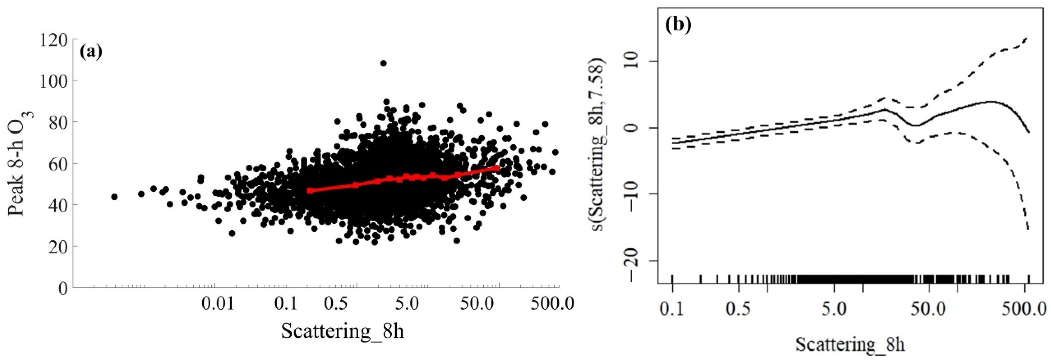
| 2 | 4 | Scattering_8h (Mm−1) | 8 h average aerosol scattering |
| 2 | 5 | CO_8h (ppb) | 8 h average carbon monoxide |
| 2 | 6 | WV_8h (g kg−1) | 8 h average water vapor mixing ratio |
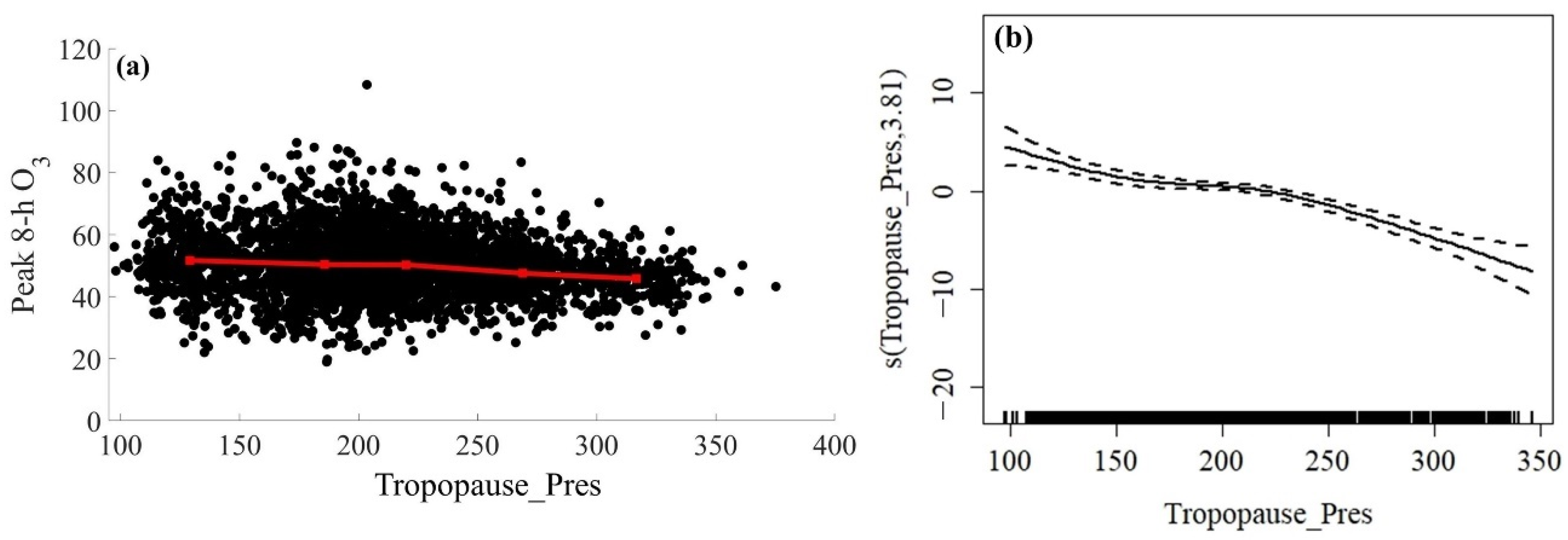
| 3 | 7 | Tropopause_Pres (hPa) | Daily, satellite-derived regional tropopause pressure |
Publisher’s Note: MDPI stays neutral with regard to jurisdictional claims in published maps and institutional affiliations. |
© 2022 by the authors. Licensee MDPI, Basel, Switzerland. This article is an open access article distributed under the terms and conditions of the Creative Commons Attribution (CC BY) license (https://creativecommons.org/licenses/by/4.0/).
Share and Cite
Ninneman, M.; Petropavlovskikh, I.; Effertz, P.; Chand, D.; Jaffe, D. Investigation of the Parameters Influencing Baseline Ozone in the Western United States: A Statistical Modeling Approach. Atmosphere 2022, 13, 1883. https://doi.org/10.3390/atmos13111883
Ninneman M, Petropavlovskikh I, Effertz P, Chand D, Jaffe D. Investigation of the Parameters Influencing Baseline Ozone in the Western United States: A Statistical Modeling Approach. Atmosphere. 2022; 13(11):1883. https://doi.org/10.3390/atmos13111883
Chicago/Turabian StyleNinneman, Matthew, Irina Petropavlovskikh, Peter Effertz, Duli Chand, and Daniel Jaffe. 2022. "Investigation of the Parameters Influencing Baseline Ozone in the Western United States: A Statistical Modeling Approach" Atmosphere 13, no. 11: 1883. https://doi.org/10.3390/atmos13111883