Lichenometric Dating and Its Limitations and Problems: A Guide for Practitioners

Abstract

Lichenometry, a method for dating rock surface exposure mainly in high latitudes and mountain environments, is based on estimates of lichen growth rates, but over the last 70 years it has been severely criticised. Its chief limitation is its questionable reliability due to three main problems: the species belonging to the Rhizocarpon subgenus, most often used by lichenometrists, are hard to identify; growth studies have highlighted the intrinsic variability of growth both seasonally and annually, with species sensitively responding to a wide range of environmental factors; and the same sensitive dependence also applies to the time taken for colonization on fresh rock surfaces. These problems cast doubt on many absolute dating studies and critics have suggested that, at best, the technique should only be used for relative dating. This paper provides guidance on identification procedures and suggests alternative dating methods based on lichen size-frequency distributions and cross-dating with other lichen species, thus avoiding reliance on a single species or support from other methods. With appropriate development, it is hoped that these approaches can provide a way forward that allows the technique to contribute more reliably to the dating of rock surfaces in regions where there are few other dating options.

1. Introduction

Lichenometric dating, initially developed by Beschel in the 1950s and now widely used by geographers, geologists, and archaeologists, is based on establishing cumulative growth rates for lichen species growing on surfaces exposed at unknown dates [1,2]. It has been used to date shrinking lake levels, trimlines, palaeofloods, structures, archaeological features, rockfalls, debris flows, volcanic events and earthquakes, landslides, glacial deposits, snow avalanching and the former extent of permafrost or persistent snow cover. As well as absolute dating, relative dating, involving measurement of whole lichen populations and construction of size-frequency distributions, has been used to identify deposits of different ages.

Beschel’s original assumptions are (1) that the size of a lichen can be directly correlated with age; (2) colonization occurs soon after rock surface exposure; (3) the largest specimens are founder members of their population and (4) growth rate differences caused by environmental variations are minimized by selection of the largest thalli, which will be growing in optimal environments. The questionable nature of these assumptions has led to a proliferation of sampling and analytical procedures in attempts to improve the reliability of the technique. Nevertheless, uncertainty remains unless there is reliable supporting evidence for dating estimates. There are still too many unsubstantiated claims as to its accuracy and dating range and, all too often, a failure to acknowledge its inherent problems.

This paper largely avoids going over the ground covered by numerous critical reviews [3,4,5,6,7,8,9,10,11,12,13,14]. The intention here is to provide a commentary and background information to help practitioners come to a clearer understanding of the technique and suggest possible future directions.

2. Problems

Section 2.1: Lichen species are notoriously difficult to identify for the non-botanist. Section 2.2: Growth rates vary widely, even neighbouring same-size individuals may show different rates both seasonally and annually. Section 2.3: The length of time taken for colonization of a freshly exposed rock surface needs to be assessed for each dating estimate. Section 2.4: Timespans (for absolute dating) need reliable verification. Section 2.5: Varying measurement techniques have been used in attempts to overcome the problems including several photographic approaches and Section 2.6: statistical procedures (including probabilities) have been employed.

2.1. Lichen Identification

Lichens are generated from a symbiotic relationship between a fungus and a photobiont (commonly an alga) together forming a thallus consisting of varying proportions of fungal and photobiont cells. There are a number of basic forms: leprose, filamentous, foliose, fruiticose, squamulose placodioid and crustose. Innes [5] gives a description of the saxicolous crustose forms belonging to the yellow-green Rhizocarpon subgenus containing the species most often used by lichenometrists. The subgenus includes four different sections. Section Rhizocarpon species are the most numerous (~24 species); then section Viridiatrum (8 species, of which 7 are parasitic on other lichens), followed by section Superficiale (8 species, with 3 parasitic) and lastly section Alpicola (only 3 species). All are prefixed with the genus name Rhizocarpon followed by the species name and, in some cases by the subspecies (ssp). For example, there are three Rhizocarpon geographicum subspecies:

R. geographicum ssp. geographicum (widespread, montane, snowpatches),

R. geographicum ssp. diabasicum (widespread).

R. geographicum spp. prospectans (Scotland, coastal northwest Europe and montane),

A synoptic key for the yellow-green Rhizocarpon, giving spore sizes, chemical reactions, characteristics of the areoles (islands forming the main thallus of crustose lichens) and apothecia (the fruiting bodies), rock types and locations, has been produced by Winchester [15] to allow for easy cross-referencing (Table S1, Supplementary Material online). The key, mostly arranged by maximum spore length, conflates the range of species characteristics as supplied in previous keys [16,17,18,19,20,21]. The range of characteristics is due to the Rhizocarpon group being notoriously variable, as illustrated by the numbers of different forms of apothecia and areoles provided in the key for each species. Only the spore sizes, areoles and chemical tests of the 15 species described by Roca-Valiente et al. [22] are not conflated.

The only way to deal with identification uncertainties for lichenometrists in the field (using a hand lens) is to record descriptions of the thallus morphology (based on the symbols in the key) and with a blade to collect a few apothecia and areoles from the centre of the thallus for chemical testing in the lab, microscopic examination and measurement of spore sizes using a microscope graticule: for a ×10 objective lens, multiply 1 ocular unit by 11.6; for ×40 multiply by 2.9, and for ×100 multiply by 1.26.

Benedict [23] helpfully describes chemical applications for the lichenometrist. Guides for chemical testing, appropriate procedures, and precautions have been produced by Bungartz [24] and Orange et al. [25]. All these procedures may be grasped, with a little practice. Confirmation by an experienced professional lichenologist should also be sought and specimens retained and deposited in a recognised herbarium.

All but one of the Superficiale (R. effiguratum, found in the Alps, southern Europe and the Rockies) have small spores as do all but 2 of the Viridiatrum (the 2 found in S. Europe). Unlike section R. geographicum which all show a strong blue reaction to iodine solution (which can be applied in the field), R. alpicola has a negative (null) reaction; this reagent can be bought as Lugol’s iodine solution or can be made by dissolving 0.5 g of iodine and 1.5 g of potassium iodide in 100 mL of distilled water. Unfortunately, 5 of the section Superficiale species in the Arctic also show negative iodine reactions so additional microscope work may be necessary). Any species that are parasitic (i.e., 7 of the Viridiatrum, 5 of the Superficiale and 1 Rhizocarpon subspecies growing in the Alps) should be avoided. And, as can be seen from their distributions, only two of the above R. geographicum ssp. need concern people working in temperate and cold environments, but that still leaves ~7 other section Rhizocarpon species to identify in cold environments.

There may be some evidence that spore sizes are an indication of growth rates among the Rhizocarpon subgenus. Species with smaller spores growing in polar regions and high mountains have apparently shown quite different growth rates compared to those with larger spores. For example, several authors have found that R. alpicola (with large spores) has higher growth rates than R. geographicum [26,27]. R. lecanorinum (with the largest spores of all) grows extremely fast [28], while Luckman [29] noted that R. macrosporum (with the second largest spores) also grows to larger sizes than R. geographicum agg. on uniform-age moraines in the Canadian Rockies.

Apart from the yellow-green Rhizocarpon group, other species can be identified using guide books: Santesson [30] produced one for Sweden and Norway, Brodo [20] covered North America, and Dobson [31] produced one for British and Irish species, also relevant for other temperate regions, including descriptions and illustrations of lichen features. The same care in identification should be exercised as for Rhizocarpon.

2.2. Growth Rates and Growth Curves

Many lichenometrists have been confused by the term ‘great period’, which is defined by Beschel [2] (pp. 1045–1046) as growth tracing a sigmoidal curve with “the diameter of a thallus increasing at first very slowly… then gathering speed with many species passing through a ‘great period’ of exponential growth until the increase drops to a constant value that is maintained for a long time.” However, studies of R. geographicum have shown that the decline in lichenometric growth curves is ‘probably a methodological artefact’ [32]). This proposal was based on a study of growth and survival/mortality of populations of Rhizocarpon geographicum and Pseudophebe pubescens in Alaska [33]. They found that over time a cumulative survival probability of 1% to 2% per year could be responsible for the apparent decline into low steady growth after the so called ‘great period’. Clayden et al. [28] also found a trend of slower but accelerating growth in small R. lecanorinum thalli and faster, more nearly constant growth in larger thalli similar to that in foliose and placodioid species as modelled by Aplin and Hill [34].

Another consequence of mortality, highlighted by Loso and Doak [33], is that there is an increasing probability that older thalli are not original colonizers and that these will provide an overestimate of surface age, a fact confirmed by McCarthy [14], and that radial growth rates based on the declining curves proposed by Beschel are likely to be underestimates [28]. This also explains why the larger the search area the greater the chance of finding ever larger, longer surviving thalli.

Beschel [2] acknowledged the variability of lichen growth due to microenvironmental factors, short and long-term climate variations and species differences and he maintained that “no averaging can simplify the results”. Different approaches to data collection and analysis have attempted to overcome this problem with analysis of means based on the assumption that the longer a substrate has been exposed the greater will be the average age of the 5, or 10, largest lichens growing on it [35]. Nevertheless, without correct identification, any such dating is of questionable value unless it is certain that only a single species is involved, and even then, identification is desirable for future comparative purposes.

Many other authors have confirmed growth variability due to species differences or variations in microenvironment, temperature (and altitude), sunshine, humidity and precipitation, both seasonally and annually and even between same-sized individuals of a species on adjacent boulders [5,14,27,36,37,38,39,40,41,42,43,44,45,46,47,48]. Trenbirth and Mathews [9] in a 25-year study of Rhizocarpon growth in southern Norway found that growth of the Rhizocarpon subgenus varied, depending on location, from 0.43 to 0.87 mm yr⁻¹, with interannual variability exceeding 1.0 mm yr⁻¹ at some sites. Unfortunately, since identification was only to subgenus level, any inter-specific growth differences may have been obscured.

Despite the evidence for variable growth and uncertainty as to the form of growth curves, dating has been attempted using four different approaches. The first, used for absolute dating, is based on repeat measurements of selected specimens over an extended period, with construction of growth rate-size curves drawn around largest measurements or, alternatively, around mean annual diameter growth through time [9].

The second, an indirect approach used for the construction of growth curves, is based on comparison of two populations on surfaces of different dates. “Histograms are prepared for both sets of thalli, and comparison of the mean or modal values shows the amount of average growth that has taken place in a time period equal to the difference in ages of the substrates” Farrar [47] (pp. 151–152).

A third indirect dating approach is based on the construction of growth curves drawn around maximum diameters of a species growing on a range of dated surfaces. The resulting curve can also be used to date peak size-frequencies of undated populations. A 4-year study of Rhizocarpon prospectans growing on tombstones in north Wales used this approach to date local landslide surfaces bordering a road, with dating confirmed by historical evidence [48]. There would be more confidence in this approach if population size-frequency histograms could be developed for several species and their growth rates used to cross-reference the dating (see below).

The fourth approach used both for absolute and relative dating was devised by Bradwell et al. [49]. For absolute dating they constructed curves based on measurements of the longest axis of Rhizocarpon section Rhizocarpon (excluding section Alpicola) growing on securely dated surfaces in southeast Iceland. For absolute dating of surfaces, the largest lichens were projected onto the curve. For indirect dating, size-frequency graphs were generated for each of the selected fixed-area survey sites and linear regression analyses with least-squares regression was used to calculate size-frequency distributions, with dating based on the gradient of the size-frequency (log₁₀) distribution versus surface age. Bradwell et al. propose that this is a statistically robust and a more powerful technique than using the single (or several) largest lichen thalli for surfaces older than 70 years (with the minimum age limitation due to the exponential form of the age-gradient curve).

Size-frequency distributions, also widely used, are likely to display the relative age of populations [4,8,50,51,52,53,54,55,56]. The frequencies of young R. geographicum populations will show an exponential curve with colonization initially slow, then rapidly increasing. As a population ages, younger thalli numbers decrease due to competition for space and mortality and the distribution will display a log normal to negative skew; eventually mortality will reduce the frequencies and the distribution may contain gaps. Population dynamics are further explained by Loso and Doak [33].

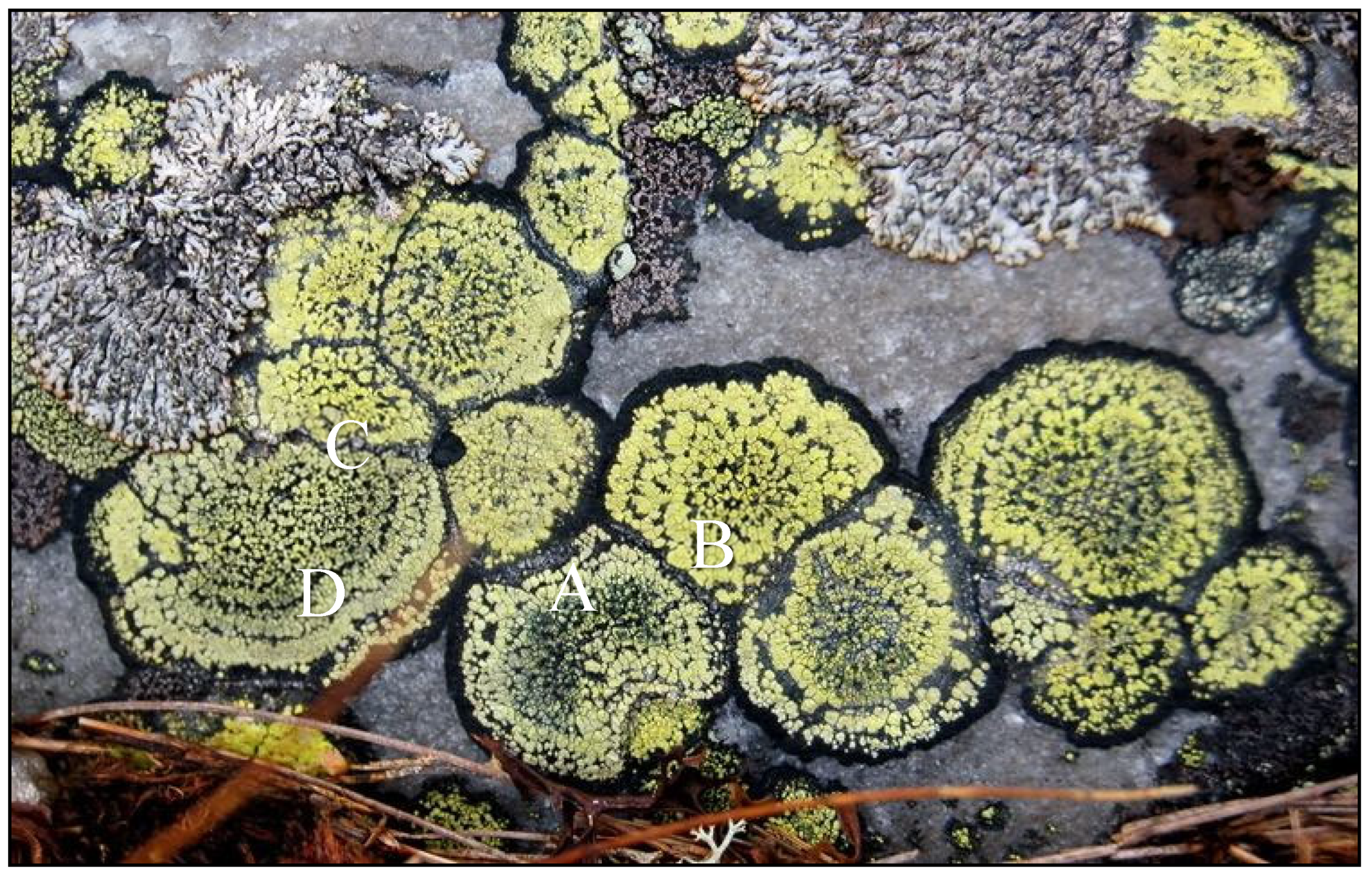
Detection of anomalously large thalli that could invalidate growth rate estimates has been the concern of many authors: this is discussed at length by Innes [5] (pp. 199–203) and McCarthy [14]. Anomalous thalli could be from an older population on a later introduced boulder or growths that have fused with section Rhizocarpon species that either lack or have an indistinct margin [28]. Figure 1 shows an example of a species, probably Rhizocarpon alpicola, with a distinct black thalline margin enclosing a broad yellow band of areoles.

There have been numerous growth studies of lichen genera other than Rhizocarpon and a logistic model for the growth rates of foliose and placodioid species was produced by Aplin and Hill [34]. Patterns of seasonal growth in foliose species, as in crustose species, have been shown to vary depending on region [57]. Where winters are severe, as in Poland [58], the Antarctic [59], and Colorado [60,61,62], lichen growth tends to occur in the summer months. Where rainfall is seasonal, distinct growth patterns may be repeated in successive years [63,64]. More complex patterns have been observed in milder environments, where maximum growth can occur in any season [65], with substantial differences from year to year [9,66].

The effect of moisture differences on the growth of section R. geographicum was also deduced by Winchester [15] working in graveyards with rainfall varying west to east across Scotland and the western Alps (Figure 2).

Figure 2. The effect of moisture differences at different latitudes on the growth of section R. geographicum, with rainfall varying wet to dry, across Scotland and the western Alps. The Chamonix curve (*) is inflated probably due to the site being on an alluvial fan (see Figure 3) [15].

Figure 2. The effect of moisture differences at different latitudes on the growth of section R. geographicum, with rainfall varying wet to dry, across Scotland and the western Alps. The Chamonix curve (*) is inflated probably due to the site being on an alluvial fan (see Figure 3) [15].

Figure 3. Arrow to cemetery on alluvial fan in Chamonix.

Figure 3. Arrow to cemetery on alluvial fan in Chamonix.

Moisture effects were also noted on a boulder beach at Bådamalen, northern Sweden. Here, on the shore, R. alpicola grows at approximately twice the rate of the species 5 km inland at Bygdeå (Figure 4), with the difference likely due to moist sea air low in salt; in the Bothnian Gulf salt content is <3‰ [67].

2.3. Colonization

Although true ecesis (colonization) should be taken from the initial synthesis of algal and fungal cells forming microscopic ‘wefts’ [12], for the purposes of the lichenometrist colonization it is based on the first visible growths [68]. Colonization, initially very slow, and varying between species, depends on environmental conditions including moisture, temperature, the length of growing season, and the degree of rock weathering [3,5,52,69,70]. Any aggregation of species could obscure between-species differences and add a further measure of doubt to absolute dating [10].

Winchester and Sjoberg [67] provide some examples of varying colonization rates in northern Sweden. They found that R. alpicola takes 8 years to colonise on beach ridges impacted by ice in the Bothnian Gulf, 12 years 5 km inland at Bydgeå, and 20 years at Bureå. Whereas section Rhizocarpon colonization on gravestones across Lappland occurred after 2 years on the opposite east to west shores at Gammelstadt and Narvik, 6 years at Røkland and Rognan some kilometres from the Atlantic shore, and also inland at Kiruna. 530 m a.s.l [15] and, according to Karlén [71], 15 years, at Tarfala a research station at the foot of Mt Kebnekaise (1130 m a.s.l). In Scotland, Winchester [15] recorded section Rhizocarpon taking 2 years to colonize at Roybridge, but 8 years at Laggan bridge lying 40 km to the east along the Spey valley where the altitude is the same, but precipitation is less than half that at Roybridge. In the western Alps, colonization was 2 years in Chamonix, and 4 years in Argentiere, Les Houches and Martigny, with difference here likely to be less related to precipitation than to the siting of the Chamonix cemetery on an alluvial fan (Figure 3). In the Tatra mountains, initial colonization by Rhizocarpon geographicum (identified only to group level) took place after 5 years and was predominantly linked to moisture [68]. The colonization periods, cited above, are for guidance only; they are likely to vary in the future due to climate warming; studies should always evaluate colonization delays for their specific species location, rock type and altitude (with these factors affecting weathering potential).

2.4. Timespans

Foliose species may have comparatively short lifespans, perhaps a maximum of 150 years or shorter depending on species and environment [44]. Crustose species can be longer-lived (Figure 5), maybe ~460 years in a temperate climate [72], ~680 years in the mountains [73], and 1400–1500 years in the Arctic [74,75,76]. Benedict [8] recommended setting a practical limit at 4000 to 5000 years, but the older the surface the more the possible sources of error; aged lichens are likely to have fused with conspecifics [14] or affected by competition, rock weathering, climate or other environmental changes [10], and long timespans are difficult to verify. Certainly the 11,500 years reported by Haworth et al. [40] is well outside the dating range of the technique. Dates can only be justified if validated by a reliable independent source.

2.5. Measurement

Although many crustose species tend to grow concentrically, irregularities in the surface or competition from other growths may distort their perimeters. To reduce this problem strict microenvironmental comparability, avoidance of competition and accurate species identification are needed as well as approximately circular thalli. Measurement methods have included rulers (accurate to ±1 mm) and callipers (accurate to ±0.01 mm and employed in direct growth measurement).

Measurement of the largest inscribed circle was recommended by Beschel [2] and later by Locke et al. [4], but when dealing with less than circular growths. This will not supply a measure of growth, only the effect of local limitations, including the direction of slope wash [3,5]. Measurement of the longest axis has been used ‘traditionally’. Alternatively, longest and/or shortest axes of 5 or 10 largest lichens have been averaged (but the shortest axis is unrepresentative of growth for the reason given above). Innes [5] discusses these approaches at length, but they all suffer if lichen identification is lacking [10,11].

Photogrametric methods for measurement [77] have included tracing on acetate the outlines of photographed thalli and digital analysis of pixel coverage. A photographic imagery approach together with processing tools and methodologies for area measurement has been developed by McCarthy [14] and Guedes et al. [78]. This method is based on repeat modelling using the Structure from Motion’ (SfM) technique using digital photogrametry, but unless accurate identification is achieved, this approach cannot reach its full potential. Hooker and Brown [79] describe the use of photographic measurements with methods for correction of magnification and parallax errors.

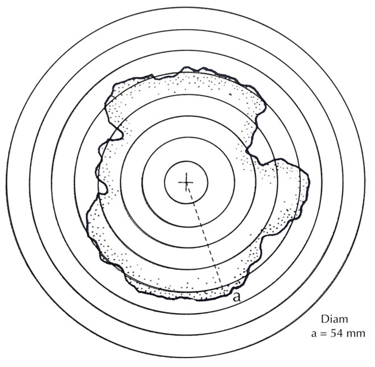
A further method is the use of clear acetate film inscribed with 5 mm concentric circles. This can be fitted over a thallus and the radius to nearest millimetre judged by eye (Figure 6). The advantage is that the film can be adjusted over less-than-flat rock surfaces, or around gravestone corners; it is particularly useful for highlighting the presence of anomalous thalli or the measurement of thalli where a section of the perimeter is missing (D in Figure 1). A test of the technique’s accuracy carried out against a photogrammetric method showed an error of ±1 mm [80]. The disadvantage of this approach is that it cannot be used for growth rate studies of very slow growing species.

2.6. Statistical Techniques

The fixed area largest lichen (FALL) method uses maximum diameters of largest lichens from 100(+) sample areas each of ~1 m² or less, with identical colonization and growth conditions. Measurements are displayed in probability density plots and histograms [81,82], but Osborn et al. [10] (pp. 9–10), although crediting its potential, raised questions concerning this approach as did McCarthy [14].

Other complex statistical procedures have been devised: (1) the Generalized Extreme Value (GEV) group [6,83,84] averages the axes of the largest lichens then models the distribution of all the lichen measurements using a Bayesian approach and GEV value distribution theory. (2) The U² technique, proposed by Orwin et al. [85], is a method for distinguishing between unimodal populations with marked differences in size-frequency gradients. Neither of these approaches meet the stringent requirements put forward by Osborn et al. [10].

3. Supportive Independent Dating Methods

Where there are no historical records, dendrochronology is the technique most frequently used for supportive dating [86]. This is effective where there are trees on or flanking the surface to be dated: for example, the age of a landslide could be indicated by the first tree ring to show damage or reaction wood. However, where trees have regrown following ice retreat there is always the question of the length of time before ecesis (which may not be the same as the time taken for lichen colonization [10] plus the number of years growth to coring height. A firm date may be achieved if, where wood has been buried, its subfossil ring widths can be cross-dated with those of nearby surviving trees [73]; older trees can also be used to assess the effects of climate change on lichen growth rates over time, although climate analysis may be complicated if trees are growing on slopes [87,88]. Innes [5] notes a number of studies based on colonization delays for various tree species and he also lists species with irregular growth rings that are unsuitable for lichenometric comparison.

Tephrochronology, where there are volcanics, could be useful for validating lichenometric age estimates over a few hundred years [89,90]. A critical review comparing lichenometric dating most unfavourably with tephrochronological ones has been provided by Decaulne [13].

Cosmogenic dating, based on beryllium-10 (¹⁰Be), may be useful where longer time frames are needed [76,91]. It has been used in Alaska [88] to provide independent minimum ages for rocks with exposure exceeding 1000 years. Stone [63] details the need for necessary scaling factors to compensate for local variations in cosmic ray flux and Heyman et al. [92] note the possibility of age overestimation.

Radiocarbon (¹⁴C) dating of buried trees and soils underlying moraines has been widely used, but organics in soil samples may be contaminated (particularly those from under moraines) and give dates that are too old [42,93]. Locke et al. [4] (pp. 26–27) write at length about the problems using radiocarbon ages for dating deposits. It should also be remembered that lichens supply minimum dates whereas ¹⁴C dating provides maximum dates and a need for calibration due to atmospheric fluctuations over time.

A further approach, percentage cover has been employed as a relative dating technique to investigate lichen succession [94]. It has been used to fill in unknown dates on moraine sequences and evaluate the importance of snow cover and aspect [60,61,95]. It is based on the assumption that the percentage of the surface area of a boulder covered by lichens increases through time. Both the maximum percentage cover on any one boulder and the mean percentage cover on all boulders on a substrate have been used [4]. The results of published studies suggest that percentage cover measurements may have some potential for relative and absolute dating [5].

4. Ways Forward

4.1. Population Size-Frequency: Absolute and Relative Dating

Analysis of size-frequencies can provide insights into events and micro-environmental effects and reveal the age-order and stability of a deposit and differing colonization rates on surfaces of different aspects, with the possibility of dating specific events where there is reliable supportive dating and accurate species identification. Further work needs to be done to investigate the effect on size-frequency distribution shapes of different size class intervals.

Size-frequency approaches can be used for both absolute and relative dating; these require sampling surfaces of similar size, slope angle, aspect and lithology and use of the longest axial measurements of all thalli in a population, with a population containing not less than thirty individuals, but ideally 100 to <1000 and statistical tests can be used to show where smaller populations may safely be grouped. The approaches used by Loso and Doak [33] are highly recommended.

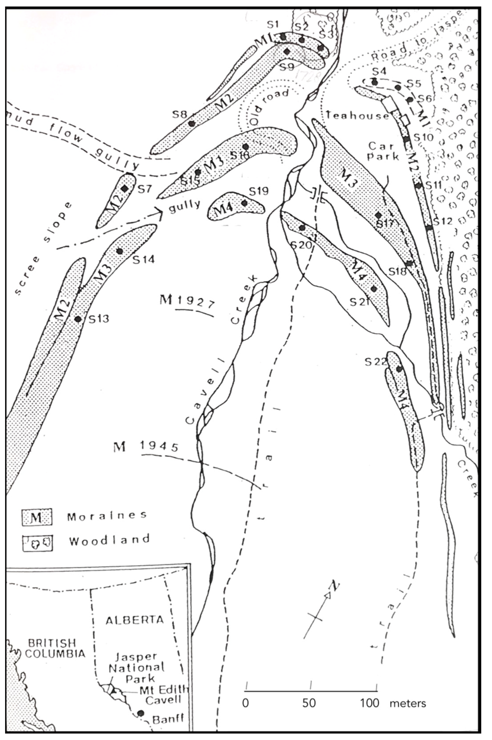
A development of relative dating using the size-frequency approach was carried out by Nick Gough in 1989 for his undergraduate dissertation at the School of Geography, Oxford University (unpublished [96]). The selected field area was Mt Edith Cavell, USA and data were collected from the four oldest moraines deposited by the Cavell glacier (Figure 7). These had previously been dated by Heusser [97] and Luckman [29], with dating validated using tree rings and historically dated surfaces. Gough, focusing on Rhizocarpon geographicum to coincide with Luckman’s data, used a random stratified dating approach, with strict attention paid to microenvironmental comparability. Thalli on ridge crests with flat or near flat boulders were sampled at 30 m intervals, with 22 quadrats of 2 m × 2 m and boulders under 50 cm diameter excluded. Sample numbers varied between 50 and 109 and a total of 1679 thalli were measured down to a minimum of 5 mm using the concentric rings method to the nearest 1 mm.

One-way analysis of variance was used to show relative differences between the Cavell moraine sample means with 95% confidence intervals (Figure 8). This approach deals with detection of different generations on a moraine [13]. The mean and standard deviations of such mixed populations should distinguish mixed from uniform populations.

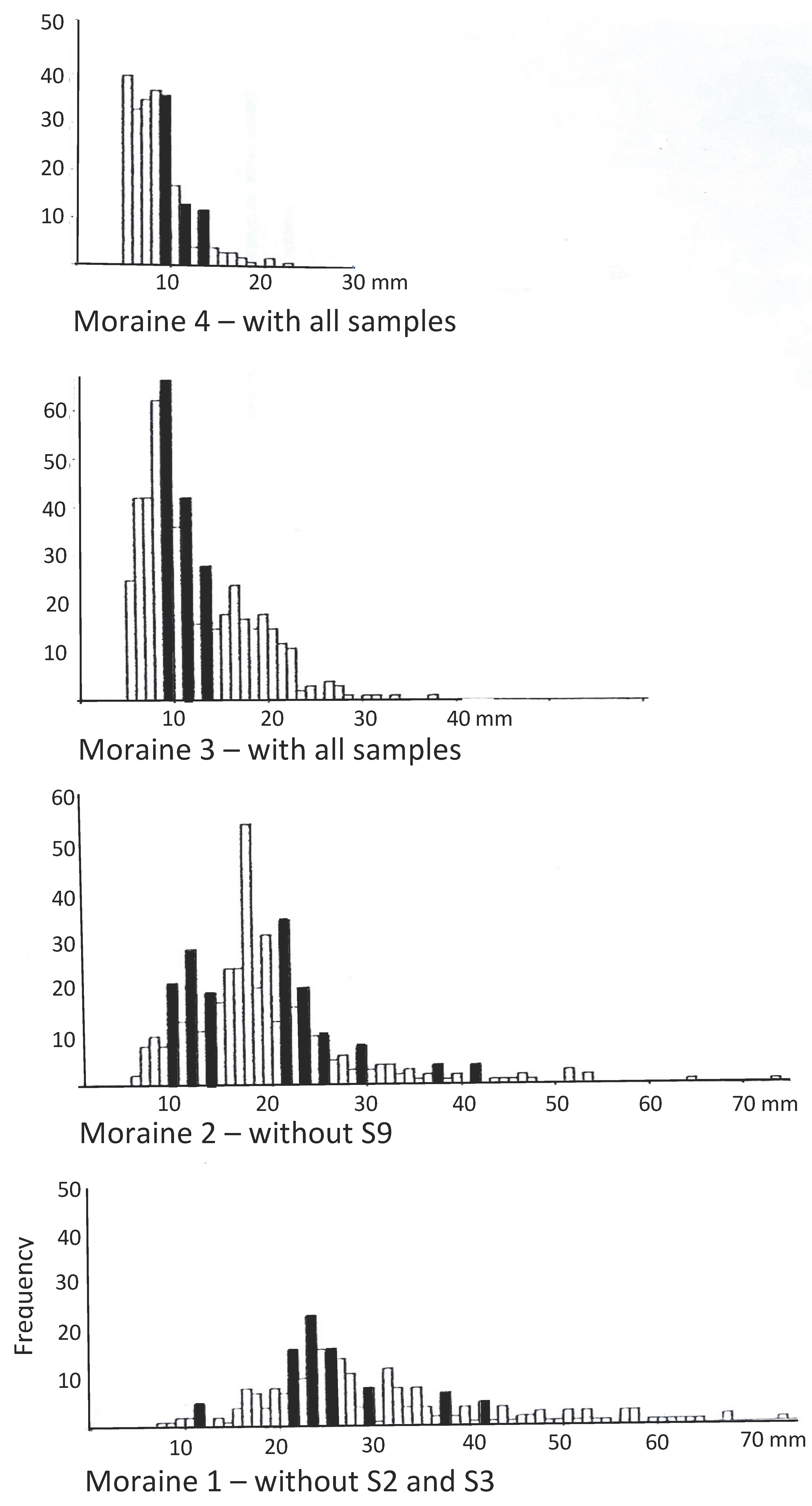
Examples of this possibility are shown by three of the 22 sampling sites on the four Cavell moraines: two (S2 and S3) on the oldest moraine 1, and one (S9) on moraine 2. The map shows these grouped together; S2 and S3 have means suggesting that they could be part of moraine 2 while S9 spans the time interval between moraines 2 and 3, possibly caused either by disturbance from a small section of old road between the moraines or mixed populations, or could this be evidence for measurements of anomalous large growths of R. macrosporum mentioned as present by Luckman [29]? The histograms for the combined samples for each moraine (with ‘misfit’ samples excluded) show ageing Poisson distributions (Figure 9).

Similar peaks in the size-frequency distributions across the four moraines suggest uniformly raised colonization episodes (Figure 10). If these patterns can be linked with local tree ring patterns, this could provide additional information on climatic variations.

The Mt Edith Cavell moraines were also used as a dating exercise by McCarthy [14] following a 20-year study of Rhizocarpon geographicum agg. growth. He indirectly estimated growth rates by dividing the means of the long axis of his five largest thalli by the age of their historically dated surfaces. Despite lack of precise identification, similar results were obtained when compared with Luckman’s dating [29].

4.2. Lichen Species Cross-Dating

A dating framework can be obtained by cross-referencing the growth rates of different species. Although this approach lacks independence due to the construction of growth curves based on species growing on dated surfaces, the uncertainties implicit in the initial assumptions are less important since the size of the confidence interval and the standard deviation of the mean should indicate the reliability or otherwise of the results. Surprisingly, despite a number of studies that have produced growth rates for many species or that have suggested species other than Rhizocarpon for use in lichenometry [4,43,77,98,99]. Only Winchester [80], Bull [82] and Lindsay [100] have applied cross-dating as an independent method for achieving absolute dating estimates.

To test this approach, a cross-dating exercise was carried out at Avebury, a stone circle in Wiltshire [80]. Eleven logistical growth curves [101] (pp. 176–177) were constructed from radial measurements of largest lichens including both foliose and crustose species growing on gravestones and marker posts erected by archaeologists. Six of these species were used to find a date for boulders dragged out of a field by a local farmer to line the banks of a nearby river. When the farmer was contacted, he revealed that the cross-dated mean (the logistical curves provided a better fit for the growths than curves drawn by eye) was accurate almost to the month, with a standard deviation of 1.72 years. The timespan was very short (19 years) and the dating obtained was from the exponential period of the species’ growth (Figure 11). Dating over a longer time frame could show a larger standard deviation. Bull [82] gives some indication of the size of error term using two pairs of unrelated species to date seismicity on the San Andreas Fault system, with dating showing a standard error of ±2.4 over 300 years and ±16 over 1200 years.

It makes sense to validate lichen dates by cross-dating with a range of different lichen species (the more the better) to support determinations-rather than use alternative dating techniques all with their own provisos. More cross dating studies using multiple species, whether based on growth curves for single largest lichens or means of five largest lichens, are needed to test the reliability and timespan of this approach. In particular it could be useful to investigate whether, with increasing time, such indirectly constructed growth curves provide overestimates of age. The time span in the Avebury study was too short to illustrate this.

5. Conclusions

Although the reviews of Jochimsen [3], Locke [4], and Innes [5] were published long ago, lichenometric dating still provides questionable results and the critical review by Osborne et al. [10] remains valid. Decaulne [13] provides advice on procedures for future lichenometrists to follow. Among the potential problems for the technique are the difficulty of correctly identifying species, variable growth rates, estimation of colonization delay and difficulties in evaluating timespans. The use of varying measurement techniques and complicated statistical procedures have done little to resolve these problems.

The first essential step along the path to identification is selection of lichens that are visually strongly similar followed by a description of the thallus; the second step should be chemical testing and the third step, if chemical tests are inconclusive, is microscope work. Difficulties in identification have, in the past, often been compounded by taxonomists who have differed in their descriptions and taxonomic concepts. However, lichenometrists should not be discouraged by this. With the help of the synoptic key, herein provided, and a careful description that can be used as a reference when comparing species in the field, a working consistency may be maintained and, over time if the descriptions and voucher specimens can be stored, preferably with lichenologists or in herbaria, identification can be confirmed.

Once this problem has been overcome, for absolute dating there is the question of validating growth rates. Except for very young thalli, studies of R. geographicum have shown that a decline into constant linear growth after initial exponential increase is probably an artefact of growth curve construction due to mortality and or the fragmentation of older thalli. Fortunately for lichenometrists, since mortality is a constant factor, this should not affect dating possibilities, although it must be acknowledged that growth curves based on lichen sizes growing on dated surfaces do not represent actual growth rates. Nevertheless, the application of growth curves derived in one area to the dating of deposits in another should be avoided.

The time taken for colonization of Rhizocarpon and other species will vary [33] depending on environmental conditions and rock weathering rates, and it may also have varied in the past as a consequence of climate change. Thus, a colonization “lag” must remain, at least for older lichens, a questionable factor especially for more remote dating. Nevertheless, the current scale of potential error, up to 30 or more years in high polar environments, compared with radiocarbon or other dating techniques is insignificant and may be evaluated if lichen species can be cross-dated and means and standard deviations applied.

Realistic timespans remain to be determined, but the variability of seasonal growth due to environmental and climatic factors complicates the issue. Measurement approaches should take into account that growth limitations acting on the dimensions of a single thallus may make it unrepresentative of the species over short timespans. The development of statistical procedures may be helpful as long as these are only applied to a securely identified single species and not an amalgam of species.

The advice and information presented in this paper is intended to show that lichenometry, despite its problems, still has potential as a dating technique. Although it remains all but impossible to validate lichenometry over long timespans, cross-dating with different species may be used for absolute dating, at least over shorter timespans, but needs further research. For relative dating, the application of population size-frequency data, as long as only a single species is involved, is of unquestionable validity. With appropriate development, it is hoped that these approaches can provide a way forward for the technique, allowing it to contribute more reliably towards assessing the consequences of climate change in environments where there are few other dating options.

References

- Beschel, R.E. Lichens as a measure of the age of recent moraines. (Translated by W. Barr, republished 1973). Arct. Alp. Res. 1950, 5, 303–309. [Google Scholar] [CrossRef]
- Beschel, R.E. Dating rock surfaces by lichen growth and its application to the glaciology and physiography (lichenometry). In Geology of the Arctic; Raasch, G.O., Ed.; University of Toronto Press: Toronto, ON, Canada, 1961; pp. 1044–1062. [Google Scholar]
- Jochimsen, M. Does the size of lichen thalli really constitute a valid measure for dating glacial deposits? Arct. Alp. Res. 1973, 5, 417–424. [Google Scholar] [CrossRef]
- Locke, W.W.; Andrews, J.T.; Webber, P.J. A manual for lichenometry. Br. Geomorphol. Res. Group Tech. Bull. 1979, 26, 1–47. [Google Scholar]
- Innes, J.L. Lichenometry. Prog. Phys. Geogr. 1985, 9, 187–254. [Google Scholar] [CrossRef]
- Jomelli, V.; Grancher, D.; Naveau, P.; Cooley, D.; Brunstein, D. Assessment study of lichenometric methods for dating surfaces. Geomorphology 2006, 86, 131–143. [Google Scholar] [CrossRef]
- Bradwell, T.; Armstrong, R.A. Growth rates of Rhizocarpon geographicum lichens: A review with new data from Iceland. J. Quat. Sci. 2007, 22, 311–320. [Google Scholar] [CrossRef] [Green Version]
- Benedict, J.B. A review of lichenometry dating and its application to archaeology. Am. Antiq. 2009, 74, 143–173. [Google Scholar] [CrossRef]
- Trenbirth, H.E.; Matthews, J.A. Lichen growth rates on glacier forelands in southern Norway: Preliminary results from a 25-year monitoring programme. Geogr. Ann. Ser. A Phys. Geogr. 2010, 92, 19–39. [Google Scholar] [CrossRef]
- Osborn, G.; MacCarthy, D.P.; La Brie, A.; Burke, R. Lichenometric Dating: Science or Pseudo-Science? Quat. Researc. 2015, 83, 1–12. [Google Scholar] [CrossRef]
- Osborn, G.; McCarthy, D.P. Lichenometric dating: Science or pseudo-science? Response to comments by Michael, A. O’Neal. Quat. Res. 2016, 86, 244–245. [Google Scholar] [CrossRef] [Green Version]
- Armstrong, R.A. Lichenometric dating (lichenometry) and the biology of the lichen genus Rhizocarpon: Challenges and future directions. Geogr. Ann. 2016, 98, 183–206. [Google Scholar] [CrossRef] [Green Version]
- Decaulne, A. Lichenometry in Iceland, results and application. Géomorphologi 2016, 22, 77–91. [Google Scholar] [CrossRef] [Green Version]
- McCarthy, D.P. A simple test of lichenometric dating using bidecadal growth of Rhizocarpon geographicum agg. and structure-from-motion photogrammetry. Geomorphology 2021, 385, 107736. [Google Scholar] [CrossRef]
- Winchester, V. An evaluation of lichenometry: With Field Studies in Lappland, Britain and the Western Alps. Unpublished Thesis, University of Oxford: Oxford, UK, 1989; Volume 1–2, British Library DSC shelf mark D 170885. [Google Scholar]
- Runemark, H. Studies in Rhizocarpon I: Taxonomy of the yellow species in Europe. Opera Bot. 1956, 2, 5–152. [Google Scholar]
- Thompson, J.W. Notes on Rhizocarpon in the Arctic. Nova Hedwig. 1967, 14, 421–481. [Google Scholar]
- Wirth, V. Die Silicatflecten-Gemeinschaften in Baseseralpinen Zentral-Europa. Diss. Bot. 1972, 17, 1–306. [Google Scholar]
- Feuerer, T. Zur Kentisder Flechtengattung Rhizocarpon in Bayern. Ber. Bayer. Bot. Ges. Zur Erforsch. Der Heim. Flora 1978, 49, 59–135. [Google Scholar]
- Brodo, I.M.; Duran Sharnhoff, S.; Sharnhoff, S. The lichens of North America; Yale University Press: New Haven, CT, USA, 2001. [Google Scholar]
- Poelt, J.; Černohorský, Z.; Schaefer, J. Rhizocarpon Ram. Em. Th. Fr. Subgenus Rhizocarpon in Europe. Arct. Alp. Res. 1988, 20, 292–298. [Google Scholar] [CrossRef]
- Roca-Valiente, B.; Hawksworth, D.; Peréz-Ortega, S.; Crespo, A. Type studies in the Rhizocarpon geographicum group (Rhizocarpaceae, lichenized Ascomycota). Lichenologist 2016, 48, 97–110. [Google Scholar] [CrossRef]
- Benedict, J.B. Techniques in lichenometry: Identifying the yellow Rhizocarpons. Arct. Alp. Res. 1988, 20, 285–291. [Google Scholar] [CrossRef]
- Bungartz, F. A safe and accurate method to apply spot test chemicals to lichen thalli in the laboratory and the field. Evansia 2002, 19, 123–124. [Google Scholar] [CrossRef]
- Orange, A.; James, P.W.; White, P.J. Microchemical Methods for the Identification of Lichens; British Lichen Society: London, UK, 2001; ISBN1 0954041801. ISBN2 9780954041809. [Google Scholar]
- Innes, J.L. Use of an aggregated Rhizocarpon ‘species’ in lichenometry: An evaluation. Boreas 1983, 12, 183–190. [Google Scholar] [CrossRef]
- Matthews, J.A. Lichenometric dating: A review with particular reference to ‘Little Ice Age’ moraines in southern Norway. In Dating in Exposed and Surface Contexts; Beck, C., Ed.; University of New Mexico Press: Albuquerque, NM, USA, 1994; pp. 185–212. [Google Scholar]
- Clayden, S.R.; Pentecost, A.; Dawson, R.J.M. Growth of the lichen R. lecanorinum, with comments on Aplin-Hill and lichenometric curves. Symbiosis 2004, 37, 379–393. [Google Scholar]
- Luckman, B.H. Lichenometric dating of holocene moraines at Mount EdithCavell, Jasper, Alberta. Can. J. Earth Sci. 1977, 14, 1809–1822. [Google Scholar] [CrossRef]
- Santesson, R. The lichens of Sweden and Norway. Nord. J. Bot. 1984, 4, 716. [Google Scholar]
- Dobson, F.S. An Illustrated Guide to the British and Irish Species; Richmond Publishing Co., Ltd.: Slough, UK, 2011. [Google Scholar]
- Loso, M.G.; Doak, D.F. Lichenometry’s black box: Demographic characteristics of Rhizocarpon geographicum and Pseudephebe pubescens inferred from whole population size-frequency distributions. In AGU Fall Meeting Abstracts; American Geophysical Union: Washington, DC, USA, 2003; p. 84. [Google Scholar]
- Loso, G.M.; Doak, D.F. The biology behind lichenometric dating curves. Oecologia 2006, 47, 223–229. [Google Scholar]
- Aplin, P.S.; Hill, D.J. Growth analysis of circular lichen thalli. J. Theor. Biol. 1979, 78, 347–363. [Google Scholar] [CrossRef]
- Matthews, J.A. Families of lichenometric dating curves from the Storbreen gletschervorfeld, Jotunheimen, Norway. Nor. Geogr. Tidsskr. 2008, 28, 215–235. [Google Scholar] [CrossRef]
- Hausman, E.H. Measurements of the annual growth rate of two species of rock lichens. Bull. Torrey Bot. Club 1948, 75, 116–117. [Google Scholar]
- Orwin, J. The Effect of Environment on Assemblages of Lichens Growing on Rock Surface. N. Z. J. Bot. 1972, 10, 37–47. [Google Scholar] [CrossRef] [Green Version]
- Ten Brink, N.W. Lichen growth rates in west Greenland. Arct. Alp. Res. 1973, 5, 323–331. [Google Scholar] [CrossRef]
- Proctor, M.C.F. Sizes and growth-rates of thalli of the lichen Rhizocarpon geographicum on the moraines of the Glacier de Valsorey, Valais, Switzerland. Lichenologist 1983, 15, 249–261. [Google Scholar] [CrossRef]
- Haworth, L.A.; Calkin, P.E. Direct measurement of lichen growth in the central Brooks Range, Alaska, U.S.A., and its application to lichenometric dating. Arct. Alp. Res. 1986, 18, 289–296. [Google Scholar] [CrossRef]
- Rogerson, R.J.; Evans, D.J.A.; McCoy, W.D. Five-year growth of rock lichens in a low-arctic mountain environment, northern Labrador. Géogr. Phys. Quat. 1986, 15, 85–91. [Google Scholar] [CrossRef] [Green Version]
- Matthews, J.A. ‘Little Ice Age’ glacier variations in Jotunheimen, southern Norway: A study in regionally controlled lichenometric dating of recessional moraines with implications for climate and lichen growth rates. Holocene 2005, 15, 1–19. [Google Scholar] [CrossRef]
- Sancho, L.G.; Pintado, A. Evidence of high annual growth rate for lichens in the maritime Antarctic. Polar Biol. 2004, 27, 312–319. [Google Scholar] [CrossRef]
- Armstrong, R.A.; Bradwell, T. Growth of foliose lichens: A review. Symbiosis 2011, 53, 1–16. [Google Scholar] [CrossRef]
- Hill, D.J. The growth of lichens with special reference to the modelling of circular thalli. Lichenologist 1981, 13, 265–287. [Google Scholar] [CrossRef]
- Hill, D.J. The effect of meteorological conditions on growth in the lichen Diploicia canescens. Br. Lichen Soc. Bull. 2014, 114, 29–37. [Google Scholar]
- Farrar, J.F. A method for investigating lichen growth rates and succession. Lichenologist 1974, 6, 151–155. [Google Scholar] [CrossRef]
- Winchester, V.; Chaujar, R.K. Lichenometric dating of slope movements, Nant Ffrancon, north Wales. Geomorphology 2002, 47, 61–74. [Google Scholar] [CrossRef]
- Bradwell, T.; Dugmore, D.J.; Sugden, D.E. The Little Ice Age glacier maximum in Iceland and the North Atlantic Oscillation: Evidence from Lambatungnajökull, southeast Iceland. Boreas 2006, 35, 61–80. [Google Scholar] [CrossRef] [Green Version]
- Benedict, J.B. Recent glacial history of an alpine area in the Colorado Front Range, U.S.A. 1. Establishing a lichen growth curve. J. Glaciol. 1967, 6, 817–832. [Google Scholar] [CrossRef] [Green Version]
- Benedict, J.B. Arapaho Pass. In Glacial Geology and Archeology at the Crest of the Colorado Front Range; Center for Mountain Archeology: Ward, CO, USA, 1985; pp. 1–197. [Google Scholar]
- Innes, J.L. Size frequency distributions as a lichenometric technique: An Assessment. Arct. Alp. Res. 1983, 5, 417–424. [Google Scholar] [CrossRef]
- McCarroll, D. A new approach to lichenometry: Dating single age and diachronous surfaces. Holocene 1994, 22, 383–396. [Google Scholar] [CrossRef]
- Caseldine, C.J.; Baker, A. Frequency Distributions of Rhizocarpon geographicum s.l., Modeling, and Climate Variation in Triillaskagi, Northern Iceland. Arct. Alp. Res. 1998, 30, 175–183. [Google Scholar] [CrossRef]
- Bradwell, T. Glacier Fluctuations, Lichenometry and Climate Change in Iceland. Ph.D. Thesis, University of Edinburgh, Edinburgh, UK, 2001. Available online: https://www.researchgate.net (accessed on 1 September 2022).
- Bradwell, T. Lichenometric dating in southeast Iceland: The size-frequency approach. Geogr. Ann. 2004, 86A, 31–41. [Google Scholar] [CrossRef]
- Armstrong, R.A. Growth rate measurements of Rhizocarpon geographicum in the Snoqualimie Pass, Washington, USA. Arct. Antarct. Alp. Res. 2005, 37, 411–415. [Google Scholar] [CrossRef] [Green Version]
- Rydzak, J. Investigations on the growth rates of lichens. Ann. Univ. Mariae Curie-Sklodowska Sect. C 1961, 16, 1–15. [Google Scholar]
- Hooker, T.N. Factors affecting the growth of Antarctic crustose lichens. Br. Antarct. Surv. Bull. 1980, 53, 1–19. [Google Scholar]
- Benedict, J.B. Experiments on lichen growth, I. Seasonal patterns and environmental controls. Arct. Alp. Res. 1990, 22, 244–254. [Google Scholar] [CrossRef]
- Benedict, J.B. Lichen mortality due to late-lying snow: Results of a transplant study. Arct. Alp. Res. 1990, 22, 81–89. [Google Scholar] [CrossRef]
- Benedict, J.B. Experiments on lichen growth, II. Effects of a seasonal snow cover. Arct. Alp. Res. 1991, 2, 189–199. [Google Scholar] [CrossRef]
- Stone, J.O. Air pressure and cosmogenic isotope production. J. Geophys. Res. 2000, 105, 23753–23759. [Google Scholar] [CrossRef]
- Boucher, V.L.; Nash, T.H., III. Growth patterns of Ramalina menziesii in California: Coastal vs. Inland populations. Bryologist 1990, 93, 295–302. [Google Scholar] [CrossRef]
- Armstrong, R.A. Seasonal growth of the crustose lichen Rhizocarpon geographicum (L.) DC. in south Gwynedd, Wales. Symbiosis 2006, 41, 97–102. [Google Scholar]
- Fisher, P.J.; Proctor, M.C.F. Observations on a season’s growth in Parmelia Caperata and P. Sulcata in South Devon. Lichenologist 1978, 10, 81–89. [Google Scholar] [CrossRef]
- Winchester, V.; Sjöberg, R. Lichenometry and beach ridge formation at Bådamalen on the North Bothnian coast, Sweden. Z. Geomorphol. 2003, 47, 485–498. [Google Scholar] [CrossRef]
- Kędzia, S. Initial colonization by Rhizocarpon geographicum in the Tatra Mountains. J. Mt. Sci. 2021, 18, 407–415. [Google Scholar] [CrossRef]
- Matthews, J.A.; Trenbirth, H.E. Growth rate of a very large crustose lichen (Rhizocarpon subgenus) and its implications for lichenometry. Geogr. Ann. Ser. A Phys. Geogr. 2011, 93, 27–39. [Google Scholar] [CrossRef]
- Armstrong, R.A. The biology of the crustose lichen Rhizocarpon geographicum. Symbiosis 2011, 55, 53–67. [Google Scholar] [CrossRef]
- Karlén, W. Holocene glacier and climatic variations, Kebnekaise mountains, Swedish Lappland. Geogr. Ann. 1973, 55, 29–63. [Google Scholar] [CrossRef]
- Winchester, V. An assessment of lichenometry as a method for dating recent stone movements in two stone circles in Cumbria and Oxfordshire. Bot. J. Linn. Soc. 1988, 96, 57–68. [Google Scholar] [CrossRef]
- Larocque, S.J.; Smith, D.J. Calibrated Rhizocarpon spp. growth Curve for the Mount Waddington Area, British Columbia coastal mountains, Canada. Arct. Antarct. Alp. Res. 2004, 36, 407–418. [Google Scholar] [CrossRef] [Green Version]
- Broadbent, N.D.; Bergqvist, K.I. Lichenometric chronology and archaeological features on raised beaches: Preliminary results from the Swedish north Bothnian coastal region. Arct. Alp. Res. 1986, 18, 297–306. [Google Scholar] [CrossRef]
- Solomina, O.; Calkin, P.E. Lichenometry as applied to moraines in Alaska. U.S.A. and Kamchatka, Russia. Arct. Antarct. Alp. Res. 2003, 35, 129–143. [Google Scholar] [CrossRef]
- Young, N.E.; Briner, J.P.; Kaufman, D.S. Late Pleistocene and Holocene glaciation of the Fish Valley north-eastern Alaska range. J. Quat. Sci. 2009, 24, 677–689. [Google Scholar] [CrossRef]
- Miller, G.H. Variations in lichen growth from direct measurements: Preliminary curves for Alectoria miniscula from eastern Baffin Island, N.W.T., Canada. Arct. Alp. Res. 1973, 5, 333. [Google Scholar]
- Guedes, P.; Oliveira, M.A.; Branquinho, C.; Silva, J.N. Image analysis for automatic measurement of crustose lichens. arXiv 2022, arXiv:2203.00787. [Google Scholar] [CrossRef]
- Hooker, T.N.; Brown, D.H. A photographic method for accurately measuring the growth of crustose and foliose saxicolous lichens. Lichenologist 1977, 9, 65–75. [Google Scholar] [CrossRef]
- Winchester, V. A Proposal for a New Approach to Lichenometry; Technical Bulletin 33 Shorter Technical Methods V; British Geomorphological Research Group: London, UK, 1984; pp. 3–20. [Google Scholar]
- Bull, W.B.; Brandon, M. Lichen dating of earthquake-generated regional rockfall events, Southern Alps, New Zealand. Geol. Soc. Am. Bull. 1998, 10, 60–84. [Google Scholar] [CrossRef]
- Bull, W.B.; Dating, S. Andreas fault earthquakes with lichenometry. Geology 1996, 24, 111–114. [Google Scholar] [CrossRef]
- Cooley, D.; Naveau, P.; Jomelli, V.; Rabatel, A.; Grancher, D. A Bayesian hierarchical extreme value model for lichenometry. Environmetrics 2006, 17, 555–574. [Google Scholar] [CrossRef]
- Naveau, P.; Jomelli, V.; Cooley, D.; Rabatel, A. Modelling uncertainties in lichenometry studies with an application: The Tropical Andes (Charquini Glacier in Bolivia). Arct. Antarct. Alp. Res. 2007, 39, 277–285. [Google Scholar] [CrossRef]
- Orwin, J.F.; McKinzey, K.M.; Stephens, M.A.; Dugmore, A.J. Identifying moraine surfaces with similar histories using lichen size distributions and the U2 statistic, southeast Iceland. Geogr. Ann. 2008, 90, 151–164. [Google Scholar] [CrossRef]
- Wiles, G.C.; Calkin, P.E. Late Holocene, high-resolution glacial chronologies and climate, Kenai Mountains, Alaska. Geol. Soc. Am. Bull. 1994, 106, 281–303. [Google Scholar] [CrossRef]
- Fritts, H.C. Tree Rings and Climate; The Blackburn Press: Caldwell, NJ, USA, 1976. [Google Scholar]
- Schweingruber, F.H. Tree Rings: Basics and Applications of Dendrochronology; Kluwer Academic Publishers: Dordrecht, The Netherland, 1989. [Google Scholar]
- Kirkbride, M.P.; Dugmore, A.J. Two millennia of glacier advances from southern Iceland dated by tephrochronology. Quat. Res. 2008, 70, 398–411. [Google Scholar] [CrossRef]
- Kirkbride, M.P. Datation des moraines holocènes d’Islande par téphrochronologie un état de l’art. In Neige et Glace de Montagne, Reconstitution, Dynamique, Pratiques; Collection EDYTEM; Deline, P., Ravanel, L., Eds.; Univesité Savoie: Annecy, France, 2009; Volume 8, pp. 65–78. [Google Scholar]
- Ivy-Ochs, S.; Kober, F. Surface exposure dating with cosmogenic nuclides. Eiszeitalt. Und Ggw. Quat. Sci. J. 2008, 57, 187–254. [Google Scholar] [CrossRef] [Green Version]
- Heyman, J.; Stroeven, A.P.; Harbor, J.M.; Caffee, M.W. Too young or too old: Evaluating cosmogenic exposure dating based on an analysis of compiled boulder exposure ages. Earth Planet. Sci. Lett. 2011, 302, 71–80. [Google Scholar] [CrossRef] [Green Version]
- Matthews, J.A. Limitations of 14C dates from buried soils in reconstructing glacier variations and Holocene climate. In Climatic Changes on a Yearly to Millennial Basis: Geological, Historical and Instrumental Records; Mörner, N.-A., Karlen, W., Eds.; D. Riedel: Dordrecht, The Netherlands, 1984; pp. 281–290. [Google Scholar]
- Orwin, J. Lichen succession on recently deposited rock surfaces. N. Z. J. Bot. 1970, 8, 452–477. [Google Scholar] [CrossRef]
- Haeberli, W.; King, L.; Flotron, A. Surface movement and lichen-cover studies at the active rock glacier near the Grubengletscher, Wallis, Swiss Alps. Arct. Alp. Res. 1979, 11, 421–441. [Google Scholar] [CrossRef]
- Gough, N.C. Lichenometric Analysis of the Cavell Glacier Moraines. Unpublished Dissertation, School of Geography, University of Oxford, Oxford, UK, 1989. [Google Scholar]
- Heusser, C.J. Postglacial environments in the Canadian Rocky Mountains. Ecol. Monogr. 1956, 26, 263–302. [Google Scholar] [CrossRef]
- Calkin, P.E.; Ellis, J.M. A lichenometric dating curve and its application to Holocene glacial studies in the Central Brooks Range, Alaska. Arct. Alp. Res. 1980, 12, 245–264. [Google Scholar]
- Sancho, L.G.; Palacios, D.; Green, A.T.G.; Vivas, M.; Pintado, A. Extreme high lichen growth rates detected in recently deglaciated areas in Tierra del Fuego. Polar Biol. 2011, 34, 13–822. [Google Scholar] [CrossRef]
- Lindsay, D.C. Estimates of lichen growth rates in the maritime Antarctic. Arct. Alp. Res. 1973, 5, 341–346. [Google Scholar] [CrossRef]
- Crowe, A.; Crowe, A. Mathematics for Biologists; Academic Press: London, UK; New York, NY, USA, 1969; pp. 176–177. [Google Scholar]
Figure 1.
Differing growth rates can be deduced from the shape of thalli perimeters in contact with others: (A) a small thallus showing a convex margin where it meets a larger thallus is in its rapid growth period; (B) a straight-line margin indicates equal growth rates. (C) Competition leading to thalline margins becoming less distinct and (D) a large thallus partially surrounded by smaller thalli. (Photo, with permission Arnstein Rønning).
Figure 4.
Growth curves for Rhizocarpon alpicola constructed in graveyards by the Bothnian Gulf, Sweden: at Nordingrå near Bådermalen; Bygdeå 5 km inland and 180 km to the north; and at Bureå lying on the shore 70 km further north again. Arrowed: Ytternäsan lighthouse steps repaired in 1979, construction at Bjoröklubb in 1945, and a memorial to a royal visit at Lövånger in 1921 [67].
Figure 5.
Giant Rhizocarpon alpicola of 493 mm diameter of unknown age measured in 1984 on Mt Nuolja above Abisko in Sweden [15].
Figure 6.
Measurement methods: acetate film inscribed with 5 mm concentric circles, with diameters judged by eye to the nearest 1 mm, to be fitted to the circumferences of near circular thalli and useful for detecting potentially fused thalli [80].
Figure 7.
Map of the four Mount Edith Cavell moraines adapted from Luckman (1977). Sampling sites S1 to S22 [96].
Figure 8.
One-way analysis of variance showing age-related differences between sample means (*) on the Cavell moraines, with 95% confidence intervals (in brackets) and misfit samples S2, S3 and S9 included [15].
Figure 9.
Age-related pattern of Poisson distributions on moraines of increasing age, with modes of decreasing frequency and increasing size-class as age increases [96].
Figure 10.
Size-frequency histograms for the four Cavell moraines with highlighted cross-referencing of similar class-frequencies. Similar peaks across the four moraines suggest uniformity of conditions influencing raised colonization episodes [15].
Figure 11.
Six species measured in the graveyard at Avebury (*) and used to date when boulders were moved by a farmer to line the bank of a local river [82].
Disclaimer/Publisher’s Note: The statements, opinions and data contained in all publications are solely those of the individual author(s) and contributor(s) and not of MDPI and/or the editor(s). MDPI and/or the editor(s) disclaim responsibility for any injury to people or property resulting from any ideas, methods, instructions or products referred to in the content. |
© 2023 by the author. Licensee MDPI, Basel, Switzerland. This article is an open access article distributed under the terms and conditions of the Creative Commons Attribution (CC BY) license (https://creativecommons.org/licenses/by/4.0/).
Share and Cite
MDPI and ACS Style
Winchester, V. Lichenometric Dating and Its Limitations and Problems: A Guide for Practitioners. Land 2023, 12, 611. https://doi.org/10.3390/land12030611
AMA Style
Winchester V. Lichenometric Dating and Its Limitations and Problems: A Guide for Practitioners. Land. 2023; 12(3):611. https://doi.org/10.3390/land12030611
Chicago/Turabian StyleWinchester, Vanessa. 2023. "Lichenometric Dating and Its Limitations and Problems: A Guide for Practitioners" Land 12, no. 3: 611. https://doi.org/10.3390/land12030611
Note that from the first issue of 2016, this journal uses article numbers instead of page numbers. See further details here.