
Synchronization Analysis of Christiaan Huygens’ Coupled Pendulums
Department of Mechanical and Industrial Engineering, Texas A&M University—Kingsville, 700 University Blvd., Kingsville, TX 78363, USA
Axioms 2023, 12(9), 869; https://doi.org/10.3390/axioms12090869
Submission received: 7 June 2023
/
Revised: 20 August 2023
/
Accepted: 7 September 2023
/
Published: 9 September 2023
(This article belongs to the Special Issue New Approach Development for Stability Analysis of Nonlinear Time-Dependent Dynamics)
Abstract
:This paper discovers a new finding regarding Christiaan Huygens’ coupled pendulums. The reason Christiaan Huygens’ coupled pendulums obtain synchrony is that the coupled pendulums are subject to a harmonic forcing. As the coupled pendulums swing back and forth, they generate a harmonic force, which, in turn drives the coupled pendulums, such that the two pendulums swing in synchrony once the angular frequency of the generated harmonic forcing satisfies a certain condition. The factor that determines the angular frequency of the generated harmonic forcing is the effective length of the pendulum, as its angular frequency solely depends on the length of the pendulum that swings about a fixed point. In other words, it is the effective length of the coupled pendulum that determines whether the coupled pendulum achieves synchrony or not. The novelty of this article is that the author explains and analyzes the synchronization behaviour of Christiaan Huygens’ coupled pendulums from the frequency and harmonic-forcing perspectives.
MSC:
92B251. Introduction
The study of synchronization initially started with Christiaan Huygens’ coupled pendulums; since then, different topics related to synchronization have been raised [1,2,3,4,5,6]. For example, the stability of a particular synchronization state is studied in [7,8,9] through looking at the eigenvalues of the Jacobian matrix of the linearized system; the question “is it stable once they get sync” is addressed—i.e., whether the incoherent state of coupled oscillators is stable or not. A more recent study regarding the stability of a certain synchronization state is presented in [10,11]; a remodeling of Huygens’ coupled pendulums is conducted in [12] through a finite element approach, such that the synchronous motion is investigated analytically; the analysis of the escapement mechanism that helps the pendulums achieve synchrony is presented in [13,14,15]; and the impact of surface friction on the synchrony behaviour and outcome are analyzed in [16,17]. A coupled complex network and coupled graph are introduced in [18,19,20,21]; for example, the sparse graph that is globally synchronized, and the densest graph that is not, are introduced, and the tools to analyze the synchrony behaviour of two coupled oscillators are presented in [22]. A question that is closely related to the coupled pendulums, i.e., the synchronization of coupled metronomes, is investigated in many studies in the literature [23,24,25,26,27,28,29].
In many papers [30,31,32,33,34,35,36,37,38,39], for instance, in [30], authors modelled Huygens’ coupled pendulums as two pendulums connected to a movable platform, connected to a wall through a spring and damper. We believe, however, that this model is far from the real Huygens’ coupled pendulums and, to some extent, it is not a correct model, because, in the real Huygens’ coupled pendulums, there is no spring (force) in the system. So, it would be an accurate model if the spring were removed, as correctly illustrated in [16]. It is worth mentioning that, to the best of the author’s knowledge, no study in the literature has identified the absolute accurate mathematical model for the Huygens’ coupled pendulums yet, as of today. It is rather a matter of how accurate and how close the model is to the real Huygens’ coupled pendulums. It should be noted that the significance of pursuing absolutely accurate models is that, without accurate models, we are not actually analyzing Huygens’ coupled pendulums, but something else. The goal in this paper is to try to understand Huygens’ coupled pendulums, and why Huygens’ coupled pendulums always reach an anti-synchronized state (180 degrees out of phase), instead of the synchronized state. In [22], the authors used the tools of contraction analysis, and created a virtual system, to analyze the synchrony behaviour of two coupled oscillators, by showing that the two systems are particular solutions of the virtual system and, if the virtual system is contracting, e.g., converges to zero, then it can be indicated that the two systems converge to zero, i.e., reach synchrony. It also looked at the one-way coupling configuration, and two-way coupling configuration. The authors extended the one-way coupling configuration to observer design and leader–follower model analysis, and noted that the observer design and leader–follower models all have an asymmetric setup. In [31], the authors showed that the coupled pendulums can be synchronized both in-phase and anti-phase (180 degrees out of phase), not just anti-phase, as in Huygens’s initial discovery. Some classic books on the subject can be found in [40,41,42,43].
The originality of this work compared to above literatures is based on the fact that this paper discovers a new finding regarding Christiaan Huygens’ coupled pendulums. The reason Christiaan Huygens’ coupled pendulums reach synchrony is that the coupled pendulums are subject to a harmonic forcing. In addition, the novelty of this article is that the author explains and analyzes the synchronization behaviour of Christiaan Huygens’ coupled pendulums from the frequency and harmonic-forcing perspectives, along with the free body diagram and Newton’s third law to, firstly, analyze all the forces acting on the moving platform and, then, through analyzing the coupled pendulums’ angular frequency and phase angle due to the harmonic forcing, to analyze the synchrony behaviour of the coupled pendulums. The author progresses from analyzing the behaviour of a single pendulum, based on the engineering vibration and wave approach, to analyzing the two coupled pendulums. In doing so, the author further used the engineering physics concept, i.e., the effect of harmonic forcing, on the coupled pendulums. The strategy that the author chose in this paper began with the author looking at two simple pendulums coupled via a spring as a starting point, in order to further analyze the case of Huygens’ coupled pendulums. The analysis of the synchronization of Huygens’ pendulums through harmonic forcing was conducted, and the discussion of the results is presented from different perspectives.
The synchronization behaviour of Christiaan Huygens’ coupled pendulums relates to frequency absorption. The term frequency absorption comes from physics [44], and its concept is that, when two systems have the same natural frequency, if one system, for example, is swinging, then it will cause the second system to swing in its natural frequency, even if we stop the first system afterwards. It is similar to power and energy transmission. The power from the first system is transferred to the second system. So, for example, as shown in Figure 1, if we let one pendulum swing, and leave the other pendulum alone, and suppose the natural frequency of the two pendulums is the same, then the second pendulum will start to swing in its natural frequency as time goes on, due to the moving platform moving back and forth, which is due to the reaction of the first pendulum (and supposing that there is little friction between the wheel and ground). The second pendulum absorbs the frequency of the first pendulum. The question is, can they achieve synchrony as time goes on?
There are two types of synchronizations; one comprises systems that synchronize themselves, and the other comprises systems that become synchronized through external control. Regarding the systems that synchronize themselves, a well-known example is the Millennium Bridge. Back in 2000, on the opening day of the bridge, people began to synchronize as they walked across the bridge, with all the people walking left and right. This is due to the fact that the bridge swung left and right, which made all the people become synced, which in turn swung the bridge left and right. This example is similar to the coupled metronome on a moving platform example [16], and the Huygens’ coupled pendulum experiment [32]. Because of the common term, i.e., the moving platform, as the moving platform swings back and forth, it makes the metronomes and coupled pendulums reach synchrony. Specifically, when the two metronomes swing back and forth on a moving platform, without external force, the reaction force or reaction frequency on the moving platform acts as a common driving term, and this common driving term is harmonic (forcing), which, in turn, drives the coupled pendulums to achieve synchrony. The phenomenon that these two pendulums influence each other, and finally reach synchrony, The phenomenon that these two pendulums influence each other, and finally reach synchrony, the case where systems synchronize themselves.
On the other hand, we can think of the coupled system that achieves synchrony by itself as essentially using control to reach synchrony, because spring coupling and derivative coupling are essentially the PD control. Without coupling (i.e., control), they will not reach synchrony if they start from different initial conditions, and if they do not have the same natural frequency. The reason they achieve synchrony is that they are coupled (i.e., controlled) in a particular way.
Regarding the systems that become synchronized through external control, we are inputting the external power and energy, and performing the work for the system, similar to the leader–follower model, where the leader will make all the followers do the same thing, i.e., reach synchrony. Under the external driving force, the driving frequency determines how the coupled pendulums swing. When the driving frequency is larger than a certain value, or in a certain range, the coupled pendulum will swing in one scenario, and when the driving frequency is smaller than a certain value, or in a certain range, the coupled pendulum will swing in a different way [44]. In other words, it is the length of the pendulum that ultimately determines whether the coupled pendulums reach synchrony or not, and how long it takes to reach synchrony when there is no external driving force. We can study the synchronization behaviour of the coupled pendulums by looking at the net frequency of the moving platform. The net frequency of the moving platform is dependent on the length of the pendulums. For example, if I hold the moving platform, and shake it in a sinusoidal way, and in a one-way coupling approach; i.e., the moving platform has no influence on the driver at all; then, in this case, the two pendulums will reach synchrony if a certain condition is met.
The organization of this paper is as follows: Section 2 provides a starting point and foundation, by looking at two simple pendulums coupled with a spring, in order to further analyze the Huygens’ coupled pendulum case in Section 3; an analysis of the synchronization of Huygens’ pendulums through harmonic forcing is presented in Section 3; Section 4 discusses the results of Section 2 from different perspectives; and conclusions are given in Section 5.
2. Second-Order System
For pendulums coupled via a spring only, and no damper, the position of one pendulum is the linear combination of two normal modes (considering there are two pendulums coupled) at any time, i.e., the superposition of the normal modes [44]. We will treat the synchrony problem as a physics problem here. To show mathematically why the spring coupling alone is not enough to achieve synchrony, we will use the following case study as a starting point, i.e., two simple pendulums coupled via a spring, as shown in Figure 2.
It is known that the general solution (i.e., the position of a pendulum) of the coupled pendulums is the superposition of the two normal modes of the coupled pendulums, as shown below:
where and are the positions of the two pendulums from the equilibrium position, as shown in Figure 2b, and are the initial positions that correspond to the two normal modes and , and are the phase angles that correspond to the two normal modes and , represents the lower mode, and represents the higher mode.
For the purpose of analysis, let one pendulum start from an initial displacement and the other one stand still; i.e., the displacement is zero; and release it and let it go, as shown in Figure 2a. In this case, the equation of motion for each pendulum can be deduced from Equation (1), and rewritten as follows:
where and are the two normal modes. The above equation essentially illustrates a beat phenomenon; as the cosine term increases, the sine terms decreases, and vice versa. From here, we can see that, just using the spring alone to couple two systems, it is impossible to achieve synchrony starting from any initial condition, unless the spring coefficient is extremely high. As, when the spring coefficient is extremely high, the term rotates very fast, in this case, we can think of the sine and cosine terms as always having approximately the same value. If the spring coefficient is not high, the term rotates very slowly, and so does the term and, therefore, it is not possible to match or synchronize it with the term .
Furthermore, a strong coupling indicates that and are far away from each other; i.e., the term is larger and, therefore, rotates faster, meaning that synchrony would be achieved faster, if they were able to synchronize. A weak coupling indicates that and are close to each other; i.e., the term is smaller and, therefore, rotates slower; i.e., synchrony would be achieved more slowly, if they were able to synchronize. To consider an extreme case, let us move the spring all the way to the top; in this way, there is no coupling (in this case ), then one pendulum swings all the time, and the other one does not.
Another example of a second-order system is the Kuramoto model for two particles, which is expressed as below:
where is the natural frequency; is either 1 or 0, and 1 means the two particles are coupled, and 0 means the two particles are decoupled; represents the position of the ith particle; and represents the position of the jth particle. It should be noted that the Kuramoto mode is a nonlinear system because of the sine term; you can also remove the sine term, and then the system becomes a linear system. The strength of the coupling matters, as illustrated in the animation of the Kuramoto model [45] and pendulums coupled via a spring, through moving the spring either up or down, as shown in Figure 2c.
3. Synchronization of Huygens’ Pendulums through Harmonic Forcing
In the case of a single pendulum that is attached to a movable platform, as shown in Figure 3, when it swings, the movable platform goes left and right, but is always 180 degrees out of phase with the pendulum. For this type of setup, it is well known that the angular frequency of the pendulum is , given that the length of the pendulum is , and it is noted that, in this case, the effective length (i.e., the length rotating about a fixed point) is ; i.e., the middle point of the pendulum is now a fixed point where it does not move, and the pendulum and the moving platform are now swinging back and forth in an opposite way about the middle point of the pendulum.
The equation of motion in the horizontal direction for the above system (including the pendulum and the moving platform) can be expressed based on Newton’s second law, , as follows:
Equation (4) represents the equation of motion for the pendulum, and Equation (5) represents the equation of motion for the moving platform. It is noted that, under the small angle approximation, the tension force T is approximately equal to the gravitational force of the pendulum [44], i.e., the term in the equation. In other words, the term is the tension force T under the small angle approximation. It is also noted that there is no motion in the vertical direction, meaning that, here, only the equation of the motion in the horizontal direction is analyzed. In the horizontal direction, based on Newton’s second law , there is only one force component in the horizontal direction, which is coming from the sign component of the tension force T; that is why, on the right-hand side of the equation , it is . It is further noted that , which contains the , and the is the movement due to the second pendulum. After rearranging the above two equations, we have:
where represents the mass of the simple pendulum, represents the mass of the moving platform, and represents the length of the pendulum. From the above equations of motion, one can clearly see the coupling between the pendulum and the moving platform.
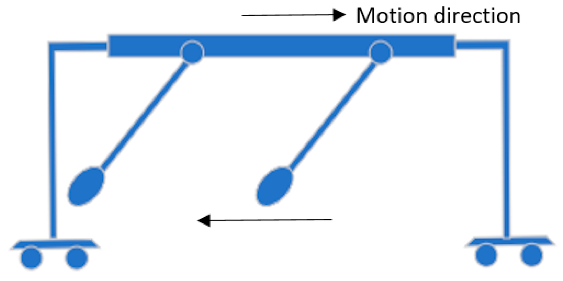
Now, we attach two pendulums to the movable platform, as shown in Figure 4b, which are the remodelled Huygens’ coupled pendulums. We assume that the two pendulums are exactly the same, and the mass is concentrated at the end. The two pendulums are coupled through a moving platform. When one pendulum swings back and forth, it will create a harmonic force on the moving platform, according to Newton’s third law, which, in turn, drives the other pendulum, and this driving force can be considered as a harmonic forcing acting on the other pendulum, and vice versa.
Different harmonic forcing will generate different swing scenarios for the pendulum and, depending on the value of the angular velocity (in this case, it is the same with the angular frequency), each pendulum might swing at the same phase angle with the moving platform, or 90 degrees out of phase, or 180 degrees out of phase. Huygens’ experiment on coupled pendulums hanging from a wooden bar on two chairs, as shown in Figure 4a, is remodelled into Figure 4b. When two pendulums swing back and forth, the wooden bar shakes, and moves to the left and right. Because of this, we modelled Huygens’ coupled pendulums as two pendulums on a moveable platform attached to a wheel-base.
The equation of the motion of the first pendulum can be expressed as follows, under the influence of the second pendulum:
where is the displacement of the first pendulum due to the motion of the second pendulum, and depends on the initial condition, and is the net angular frequency of the two pendulums. We plug Equation (9) into (8) and, after rearranging the equation, we have:
During the transient stage, according to Newton’s third law, the swing of pendulum 1 will generate a reaction force on the moving platform, and this reaction force, together with the reaction force coming from pendulum 2 to the platform, is the net harmonic force that, in turn, drives pendulum 2. A free body diagram of the moving platform is also presented in Figure 4b. As the moving platform drives pendulum 2, the effective length (i.e., the length of the pendulum that swings with respect to the fixed point) of pendulum 2 changes, depending on the frequency of the reaction force (i.e., the harmonic forcing) of pendulum 1. If , then pendulum 1 will be 180 degrees out of phase with respect to the net harmonic driving force. If , pendulum 1 will be in phase with respect to the net harmonic driving force. is the net angular frequency of the coupled pendulums, is the natural frequency of the first pendulum, and is the natural frequency of the second pendulum.
In the meantime, the swing of pendulum 2 will generate reaction force on the moving platform, and this reaction force, together with the reaction force coming from pendulum 1, is the net harmonic force that, in turn, drives pendulum 1. As the moving platform drives pendulum 1, the effective length of pendulum 1 changes, depending on the frequency of the reaction force of pendulum 2. If , then pendulum 2 will be 180 degrees out of phase with respect to the net harmonic driving force. If , pendulum 2 will be in phase with respect to the net harmonic driving force.
It is noted that the angular frequency of the pendulum is constantly changing, and this is due to the fact that the effective length of the pendulum is constantly changing. This state lasts until the coupled pendulums reach a steady state. After the transient, and during the steady state, if one has the following condition satisfied, as shown in inequality condition (11), then the two pendulums will be 180 degrees out of phase with respect to the harmonic driving force; i.e., in this case the two pendulums will achieve synchrony in phase as time goes on, as shown in Figure 5.
where is the net angular frequency of the coupled pendulums, and is the natural frequency of the first pendulum, and this frequency changes as time goes on, before the pendulum reaches the steady state, because the effective length of the pendulum changes due to the effect of the other pendulum pushing the moving platform back and forth, and vice versa. is the natural frequency of the second pendulum. It is noted that, during the transient stage, , , and are all time varying, due to the effective length of the pendulum changes because of the interactions between the two pendulums. After the transient (i.e., the steady-state stage), , , and all become constant.
The above analysis is based on the scenario where there is no friction or damping force. It is conjectured that, if there is a high level of friction, then the moving platform has the tendency to stay still and, therefore, the pendulums will become anti-synced. If there is no friction, then the pendulums will reach synchrony. As indicated in [46], in-phase synchronization happens when the damping is negligible. If the natural frequencies of the two oscillators are far apart, then no synchronization occurs; i.e., when the spread of natural frequencies among multiple oscillators is large, the systems will not achieve synchrony. The spread is decreased until a certain threshold, and then synchrony starts to appear.
It is worth noting that our experiment is different from Huygens’ coupled pendulum experiment, in which the two pendulums are hanging from a bar that is connected to two chairs, and there is a large friction between the bar and the chair, so, in Huygens’ experiment, the pendulums always become anti-synced. In our experiment, the two pendulums are hanging from a moving platform, which has very little or no friction, which is why the pendulums become synced in phase. Furthermore, we know that the angular frequency of the pendulum only depends on the length of the pendulum and, therefore, under the influence of harmonic forcing, the length of the pendulum will determine how these two pendulums swing; i.e., the pendulum might swing at the same phase angle with the moving platform, 90 degrees out of phase, or 180 degrees out of phase.
To provide a depiction of how coupled oscillators synchronize, the motion of both pendulums of the coupled pendulums are analyzed. The goal is to observe whether there is any form of synchronization between both oscillators after a certain time. A simulation diagram is drawn, as follows, in order to analyze the motion of both oscillators.
The first diagram in Figure 6 describes the angular displacement of the pendulum. As can be seen, there are two lines with different colors (red and blue); each line represents a different pendulum. During the first seconds, the oscillators move erratically; however, after seven seconds, the pendulums seem to begin moving in synchrony. The duration of the motion of the pendulums is minimal, as friction is present. According to the diagrams, it can be witnessed that both oscillators are anti-phase synchronized. This means that the oscillators have the same period, but a different angular displacement.
4. Discussion
The engineering background corresponding to the physical model in this paper is that the interaction between the two pendulums means that it is suitable to use the engineering vibration and wave approach to analyze its synchrony behaviour. The author progresses from analyzing the behaviour of single pendulum attached to a moving platform based on engineering physics, to analyzing the two coupled pendulums that are attached to the moving platform, where the author used the concept of the harmonic forcing effect on the pendulums.
It is shown from Section 3 that spring coupling alone cannot make two or more systems become synchronized, unless it starts from exactly the same initial condition, i.e., either in-phase or out-of-phase. One explanation is that the energy is transferring from the kinetic energy to spring energy and vice versa when the pendulums swing back and forth, if it starts from any initial condition. So, if a spring alone can make the systems reach synchrony, then it means that the spring is not compressed or pulled; i.e., there is no spring potential energy, which contradicts the above energy-transferring phenomena. Another explanation, coming from the fact that the general solution (i.e., the position of one of the coupled pendulums) is the superposition of the two normal modes of the coupled pendulums, as previously shown in Equation (1), as follows:
where and are the positions of the two pendulums from the equilibrium position, as shown in Figure 2b; and are the initial positions that correspond to the two normal modes and ; and and are the phase angles that correspond to the two normal modes and .
As the time is in the cosine term in the above equation, and time is always continuous (not discrete), in reality, it is impossible to make and equal to each other, because the sine term and cosine are changing as time goes on. In other words, if we let , we have
Equation (13) indicates that , and this further indicates that the two pendulums are starting from the same initial condition, because the initial position that corresponds to the higher normal is zero; i.e., the second term in Equation (1) does not exist. In other words, Equation (1) has become as follows:
It is noted that the above coupled pendulums are connected through a spring, and the top ceiling is not a moving platform, compared to the previous case, where the two pendulums were connected through a moving platform.
One remark is that, for the above pendulums coupled through a spring, if we let one pendulum swing and the other one stand still, then, in this case, we will have the beat phenomenon. Under this case, if one moves the spring up (i.e., reduces the coupling), then the sine and cosine terms rotate slower, which means that the period of the beat phenomenon becomes longer, in which case, we conjecture that it takes longer to reach synchrony, if the pendulums are able to reach synchrony. If we move the spring all the way to the top, then the coupling has become zero; in this case, one pendulum will swing back and forth, and it has no impact on the second pendulum, in which case, we conjecture that synchrony will never be achieved if the pendulums are able to achieve synchrony. Finally, as we move down the spring (i.e., the coupling is stronger), the cosine and sine terms rotate faster around the unit cycle and, in this case, the period of the beat phenomenon becomes shorter, in which case, we conjecture that synchrony will be reached faster, if the pendulums are able to reach synchrony.
By using a spring alone to couple the systems, we cannot make the coupled system reach synchrony, unless the pendulums start from the same initial condition. This is true for any second- or higher-order system, but not for a first-order system. It is noted that synchronization is not applicable to the first-order system, because we will need to have at least two objects for the synchronization problem, so the system will be at least a second-order system. Hypothetically speaking, the reason that a spring alone cannot make the coupled system become synchronized unless the pendulums start from the same initial condition in second- or higher-order systems, but that this is not true in a first-order system, is that, for the first-order system, if we couple the pendulums using a spring alone, this can be considered as two systems being coupled via a spring, but the mass of the two systems is zero. This is because, if there is no mass, then there is no inertia and, therefore, if two systems swing differently initially, then the spring will force them to reach synchrony as long as the coefficient of the spring is high enough. For second-order or higher-order systems, the mass of the system is not zero anymore and, therefore, if we use a spring alone to couple the pendulums, then what will happen is that the two systems will swing in their own ways back and forth, and they will not achieve synchrony if they start from any different initial conditions, similar to a robot arm, where, if each join is connected via a spring only, the robot arm will swing back and forth.
Some experiments in the literature are able to show that, if we put two pendulums on a movable platform, and if we let pendulum 1 swing, and leave pendulum 2 to stand still, then, after the transient state, the two pendulums can reach an anti-synced state. However, in the steady state, pendulum 1’s amplitude becomes smaller, compared to its initial amplitude. This essentially represents the frequency absorption and energy transmission from pendulum 1 to pendulum 2. The initial potential energy of pendulum 1 is transferred to both pendulums’ kinetic and potential energy, but with a smaller amplitude. It is noted that the larger the amplitude, the larger the energy.
The frequency distribution among many oscillators also has an influence on the synchrony behaviour. The more distributed the frequency of the many oscillators, the more difficult it is to reach synchrony. The less distributed the frequency of the many oscillators, the easier it is to reach synchrony. To put this into practice in a political movement, for example, the more diverse the population is, the more difficult it is to achieve synchrony; i.e., the more difficult it is to govern the population. The less diverse the population is; i.e., the more clones of the system there are; the easier it is to achieve synchrony; i.e., it is much easier to govern the population. Another example is that, if all people have the same mindset (similar to the case where all the oscillators have the same frequency), then it is very easy to gather them together, and induce a collective behaviour; i.e., reach synchrony; in order to achieve a political movement. On the other hand, if all people have completely different mindsets (as in the case where all the oscillators have very different natural frequencies), then it will be very difficult to convince each one of them to form a collective political movement; i.e., it is very difficult to achieve synchrony.
5. Conclusions
In this study, we only looked at two identical and symmetrical coupled systems. What if we had many, or even an infinite number of, coupled oscillators, and those oscillators were not symmetrical? In these cases, particularly the latter one, the problem will become more complicated to analyze. If we have many, or even an infinite number of, coupled systems, then it is essentially a wave problem. Again, it depends on the driving frequency; a different driving frequency will have different waves and, therefore, it will generate synchrony if the driving frequency meets certain conditions.
The novelty of this paper is that the author explains and analyzes the synchronization behaviour of Christiaan Huygens’ coupled pendulums from frequency and harmonic-forcing perspectives, along with the free body diagram and Newton’s third law to, firstly, analyze all the forces acting on the moving platform and, then, through analyzing the coupled pendulums’ angular frequency and phase angle due to harmonic forcing, to analyze the synchrony behaviour of the coupled pendulums.
Future work will focus on the time it takes for the pendulum to achieve synchrony, and what factors determine this time. The time it takes for the pendulums to reach synchrony essentially depends on the transient state. It is noted that the general solution to the governing equation of the coupled pendulum is the sum of the special solution (i.e., the steady state solution) and the homogenous solution (i.e., the transient state solution).
Funding
This research received no external funding.
Data Availability Statement
Not applicable.
Acknowledgments
The author would like to acknowledgement financial support from the start-up professional development fund from Texas A&M University–Kingsville.
Conflicts of Interest
The author declares no conflict of interest.
References
- Joshi, S.; Sen, S.; Kar, I. Synchronization of coupled oscillator dynamics. IFAC-PapersOnLine 2016, 49, 320–325. [Google Scholar] [CrossRef]
- Chopra, N.; Spong, M.W. On exponential synchronization of Kuramoto oscillators. IEEE Trans. Autom. Control 2009, 54, 353–357. [Google Scholar] [CrossRef]
- Pisarchik, A.; Jaimes-Reategui, R.; Lopez, J. Synchronization of coupled bistable chaotic systems: Experimental study. Philos. Trans. R. Soc. A 2007, 366, 459–473. [Google Scholar] [CrossRef]
- Bharath, R. Nonlinear Observer Design and Synchronization Analysis for Classical Models of Neural Oscillators. Master’s Thesis, Massachusetts Institute of Technology, Cambridge, MA, USA, 2013. [Google Scholar]
- Ramirez, P.; Ramos, R.; Alvarez, J. Synchronization of asymmetrically coupled systems. Nonlinear Dyn. 2019, 95, 2217–2234. [Google Scholar] [CrossRef]
- Wiesenfeld, K. Huygens’s odd sympathy recreated. Soc. Politica 2017, 11, 15–22. [Google Scholar]
- Strogatz, S.; Mirollo, R. Stability of incoherence in a population of coupled oscillators. J. Stat. Phys. 1991, 63, 613–635. [Google Scholar] [CrossRef]
- Childs, L.; Strogatz, S. Stability diagram for the forced Kuramoto model. Chaos 2008, 18, 043128. [Google Scholar] [CrossRef]
- Gambuzza, L.V.; Di Patti, F.; Gallo, L.; Lepri, S.; Romance, M.; Criado, R.; Frasca, M.; Latora, V.; Boccaletti, S. Stability of synchronization in simplicial complexes. Nat. Commun. 2021, 12, 1255. [Google Scholar] [CrossRef]
- Li, Z.; Zhang, X.; Chen, W.; Wen, B. Synchronization characteristics of two vibrator-driven pendulums. Alex. Eng. J. 2023, 64, 907–921. [Google Scholar] [CrossRef]
- Li, Z.; Zhang, X.; Chen, W.; Zhang, W.; Li, C.; Wang, X.; Wen, B. Synchronization and stability characteristics of a double-pendulum coupling vibrating system driven by two vibrators. Nonlinear Dyn. 2023, 111, 12297–12318. [Google Scholar] [CrossRef]
- Ramirez, J.P.; Fey, R.H.; Aihara, K.; Nijmeijer, H. An improved model for the classical Huygens’ experiment on synchronization of pendulum clocks. J. Sound Vib. 2014, 333, 7248–7266. [Google Scholar] [CrossRef]
- Peña Ramirez, J.; Olvera, L.A.; Nijmeijer, H.; Alvarez, J. The sympathy of two pendulum clocks: Beyond Huygens’ observations. Sci. Rep. 2016, 6, 23580. [Google Scholar] [CrossRef]
- Goldsztein, G.; Nadeau, A.; Strogatz, S. Synchronization of clocks and metronomes: A perturbation analysis based on multiple timescales. Chaos 2021, 31, 023109. [Google Scholar] [CrossRef]
- Czolczynski, K.; Perlikowski, P.; Stefanski, A.; Kapitaniak, T. Synchronization of two nonidentical clocks: What Huygens was able to observe. In Selected Topics in Nonlinear Dynamics and Theoretical Electrical Engineering; Kyamakya, K., Halang, W., Mathis, W., Chedjou, J., Li, Z., Eds.; Studies in Computational Intelligence; Springer: Berlin/Heidelberg, Germany, 2013; Volume 483. [Google Scholar]
- Goldsztein, G.; English, L.; Behta, E. Coupled metronomes on a moving platform with Coulomb friction. Chaos 2022, 32, 043119. [Google Scholar] [CrossRef]
- Wu, Y.; Wang, N.; Li, L.; Xiao, J. Anti-phase synchronization of two coupled mechanical metronomes. Chaos 2012, 22, 023146. [Google Scholar] [CrossRef]
- Townsend, A.; Stillman, M.; Strogatz, S. Dense networks that do not synchronize and sparse ones that do. Chaos 2020, 30, 083142. [Google Scholar] [CrossRef]
- Belykh, I.; Hasler, M.; Lauret, M.; Nijmeijer, H. Synchronization and Graph Topology. Int. J. Bifurc. Chaos 2005, 15, 3423–3433. [Google Scholar] [CrossRef]
- Belykh, I.; Belykh, V.; Hasler, M. Generalized connection graph method for synchronization in asymmetrical networks. Phys. D Nonlinear Phenom. 2006, 224, 42–51. [Google Scholar] [CrossRef]
- Cin, A.; Magri, L.; Arrigoni, F.; Fusiello, A.; Boracchi, G. Synchronization of group-labelled multi-graphs. In Proceedings of the 2021 IEEE/CVF International Conference on Computer Vision (ICCV), Montreal, QC, Canada, 11–17 October 2021; pp. 6433–6443. [Google Scholar]
- Wang, W.; Slotine, J. On partial contraction analysis for coupled nonlinear oscillators. Biol. Cybern. 2005, 92, 38–53. [Google Scholar] [CrossRef]
- Ulrichs, H.; Mann, A.; Parlitz, U. Synchronization and chaotic dynamics of coupled mechanical metronomes. Chaos Interdiscip. J. Nonlinear Sci. 2009, 19, 043120. [Google Scholar] [CrossRef]
- Oud, W. Design and Experimental Results of Synchronizing Metronomes, Inspired by Christiaan Huygens. Master’s Thesis, Eindhoven University of Technology, Eindhoven, The Netherlands, 2006. [Google Scholar]
- Xin, X.; Muraoka, Y.; Izumi, S.; Yamasaki, T. Analysis of synchronization of n metronomes on a hanging plate via describing function method without assumption on amplitudes of metronomes. In Proceedings of the 2017 36th Chinese Control Conference (CCC), Dalian, China, 26–28 July 2017; pp. 1129–1134. [Google Scholar]
- Kuznetsov, N.V.; Leonov, G.A.; Nijmeijer, H.; Pogromsky, A.Y. Synchronization of two metronomes. In Proceedings of the 3rd IFAC Workshop on Periodic Control Systems, Saint Petersburg, Russia, 29–31 August 2007; pp. 49–52. [Google Scholar]
- Jia, J.; Song, Z.; Liu, W.; Kurths, J.; Xiao, J. Experimental study of the triplet synchronization of coupled nonidentical mechanical metronomes. Sci. Rep. 2015, 5, 17008. [Google Scholar] [CrossRef]
- Pantaleone, J. Synchronization of metronomes. Am. J. Phys. 2002, 70, 992–1000. [Google Scholar] [CrossRef]
- Xin, X.; Muraoka, Y.; Hara, S.; Izumi, S.; Yamasaki, T. New characterization and classification of synchronization of multiple metronomes on a cart via describing function method. IFAC-PapersOnLine 2017, 50, 9450–9455. [Google Scholar] [CrossRef]
- Pena, J. Huygens’ Synchronization of Dynamical Systems: Beyond Pendulum Clocks. Ph.D. Thesis, Technische Universiteit Eindhoven, Eindhoven, The Netherlands, 2013. [Google Scholar]
- Czolczynski, K.; Perlikowski, P.; Stefanski, A.; Kapitaniak, T. Huygens’ odd sympathy experiment revisited. Int. J. Bifurc. Chaos 2011, 21, 2047–2056. [Google Scholar] [CrossRef]
- Willms, A.; Kitanov, P.; Langford, W. Huygens’ clocks revisited. R. Soc. Open Sci. 2017, 4, 170777. [Google Scholar] [CrossRef]
- Francke, M.; Pogromsky, A.; Nijmeijer, H. Huygens’ clocks: ‘Sympathy’ and resonance. Int. J. Control 2020, 93, 274–281. [Google Scholar] [CrossRef]
- Ramírez, J.; Alvarez, J. Rotating waves in oscillators with Huygens’ coupling. IFAC-PapersOnLine 2015, 48, 71–76. [Google Scholar] [CrossRef]
- Senator, M. Synchronization of two coupled escapement-driven pendulum clocks. J. Sound Vib. 2006, 291, 566–603. [Google Scholar] [CrossRef]
- Ramos, I.; Ramirez, J.; Alvarez, J. Synchronous behavior in asymmetrically coupled pendulums. In Proceedings of the 2017 International Symposium on Nonlinear Theory and Its Applications, Cancun, Mexico, 4–7 December 2017; pp. 351–354. [Google Scholar]
- Ramirez, P.; Nijmeijer, H. Enforcing synchronization in oscillators with Huygens’ coupling via feed-forward control. Nonlinear Dyn. 2019, 98, 3009–3023. [Google Scholar] [CrossRef]
- Davidova, L.; Ujvari, S.; Neda, Z. Sync or anti-sync dynamical pattern selection in coupled self-sustained oscillator systems. J. Phys. Conf. Ser. 2014, 510, 012009. [Google Scholar] [CrossRef]
- Ramirez, J.P.; Nijmeijer, H. The secret of the synchronized pendulums. Phys. World 2020, 33, 36–40. [Google Scholar] [CrossRef]
- Blekhman, I.I. Synchronization in Science and Technology; ASME Press: New York, NY, USA, 1988. [Google Scholar]
- Strogatz, S. Sync; Hyperion: New York, NY, USA, 2003. [Google Scholar]
- Pikovsky, A.; Rosenblum, M.; Kurths, J. Synchronization: A Universal Concept in Nonlinear Sciences; Cambridge University Press: Cambridge, UK, 2003. [Google Scholar]
- Boccaletti, S.; Pisarchik, A.N.; Del Genio, C.I.; Amann, A. Synchronization: From Coupled Systems to Complex Networks; Cambridge University Press: Cambridge, UK, 2018. [Google Scholar]
- French, A.P. Vibrations and Waves; CRC Press: Boca Raton, FL, USA, 1971; ISBN 9780748744473. [Google Scholar]
- Kuramoto Model. Available online: https://hdietert.github.io/static/kuramoto-animation/kuramoto.html (accessed on 12 May 2023).
- Strogatz, S. From Kuramoto to Crawford: Exploring the onset of synchronization in populations of coupled oscillators. Phys. D Nonlinear Phenom. 2000, 143, 1–20. [Google Scholar] [CrossRef]
Figure 1.
A simplified model of Christiaan Huygens’ coupled pendulums.

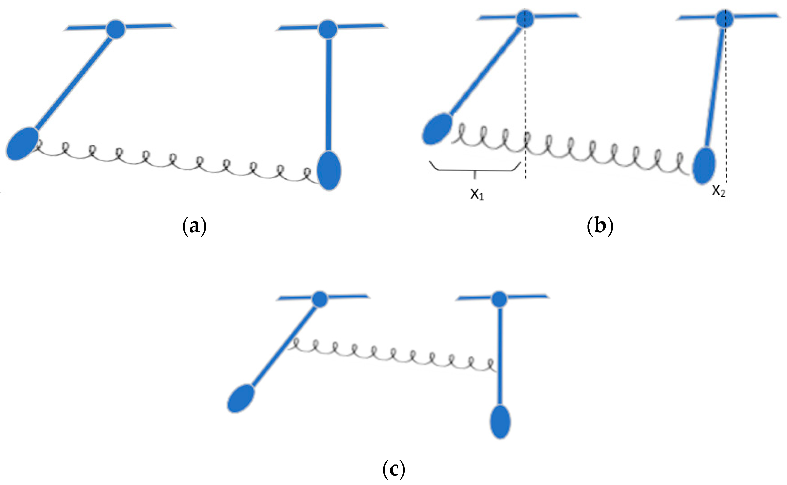
Figure 2.
Two pendulums attached to a fixed ceiling, coupled via a spring. It shows (a) initial state; (b) a random state; (c) reducing the coupling by moving the spring up.
Figure 2.
Two pendulums attached to a fixed ceiling, coupled via a spring. It shows (a) initial state; (b) a random state; (c) reducing the coupling by moving the spring up.

Figure 3.
One pendulum attached to a moving platform.

Figure 4.
Modelling of Huygens’ coupled pendulums. (a) Huygens’ coupled pendulums (b) Remodeling of Huygens’ coupled pendulums.
Figure 4.
Modelling of Huygens’ coupled pendulums. (a) Huygens’ coupled pendulums (b) Remodeling of Huygens’ coupled pendulums.

Figure 5.
Two coupled pendulums in a synced condition.

Figure 6.
Simulation diagram illustration of the oscillators’ angular displacement (degrees) and angular velocity (degrees/second) for the coupled pendulums. Two lines with different colors (red and blue), with each line representing a different pendulum.
Figure 6.
Simulation diagram illustration of the oscillators’ angular displacement (degrees) and angular velocity (degrees/second) for the coupled pendulums. Two lines with different colors (red and blue), with each line representing a different pendulum.

Disclaimer/Publisher’s Note: The statements, opinions and data contained in all publications are solely those of the individual author(s) and contributor(s) and not of MDPI and/or the editor(s). MDPI and/or the editor(s) disclaim responsibility for any injury to people or property resulting from any ideas, methods, instructions or products referred to in the content. |
© 2023 by the author. Licensee MDPI, Basel, Switzerland. This article is an open access article distributed under the terms and conditions of the Creative Commons Attribution (CC BY) license (https://creativecommons.org/licenses/by/4.0/).
Share and Cite
MDPI and ACS Style
Wei, B. Synchronization Analysis of Christiaan Huygens’ Coupled Pendulums. Axioms 2023, 12, 869. https://doi.org/10.3390/axioms12090869
AMA Style
Wei B. Synchronization Analysis of Christiaan Huygens’ Coupled Pendulums. Axioms. 2023; 12(9):869. https://doi.org/10.3390/axioms12090869
Chicago/Turabian StyleWei, Bin. 2023. "Synchronization Analysis of Christiaan Huygens’ Coupled Pendulums" Axioms 12, no. 9: 869. https://doi.org/10.3390/axioms12090869
Note that from the first issue of 2016, this journal uses article numbers instead of page numbers. See further details here.